

Pixiv - 蒼ஐ/お仕事募集中
7697 字
38 分钟
【论文阅读 | TIM 2021 | STDFusionNet:基于显著目标检测的红外-可见光图像融合网络】
STDFusionNet:基于显著目标检测的红外-可见光图像融合网络
- 题目:STDFusionNet: An Infrared and Visible Image Fusion Network Based on Salient Target Detection
- 期刊:IEEE Transactions on Instrumentation and Measurement, Vol. 70, 2021(Art. no. 5009513)
- 作者:Jiayi Ma, Linfeng Tang, Meilong Xu, Hao Zhang, Guobao Xiao
- DOI:10.1109/TIM.2021.3075747
- 代码: https://github.com/jiayi-ma/STDFusionNet
1. 摘要
- 论文提出一种基于显著目标检测(salient target detection)的红外-可见光融合网络,命名为 STDFusionNet,其目标是保留红外图像的热目标(thermal targets)与可见光图像的纹理结构(texture structures)。
- 作者引入显著目标mask(salient target mask)用于标注红外图像中“人或机器更关注的区域”,以此为不同信息的融合提供空间引导(spatial guidance)。
- 论文将显著目标mask与特定loss函数结合,用于指导特征的提取与重建;并指出:特征提取网络可选择性提取红外显著目标特征与可见背景纹理特征,重建网络融合并重建期望结果。
- 论文强调:显著目标mask仅在训练阶段需要,使得STDFusionNet在测试时是端到端模型;并且模型可隐式实现显著目标检测与关键信息融合
- 论文给出实验结论:相对“state of the arts”,其在公共数据集上可对 EN/MI/VIF/SF 指标分别取得约**1.25% / 22.65% / 4.3% / 0.89%**的提升。
2. 引言与动机
- 单一传感器/单一拍摄设置得到的图像只能从有限视角描述场景,因此融合来自不同传感器/不同设置的互补图像有助于增强场景理解;其中红外-可见光融合是重要场景之一。
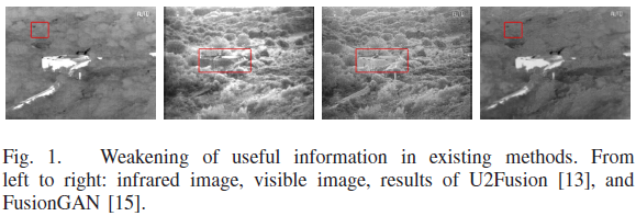
- 论文给出问题现象:一些现有融合方法会削弱“有用信息(useful information)”;并在示例中指出:U2Fusion 会弱化显著目标,FusionGAN 会弱化背景纹理。
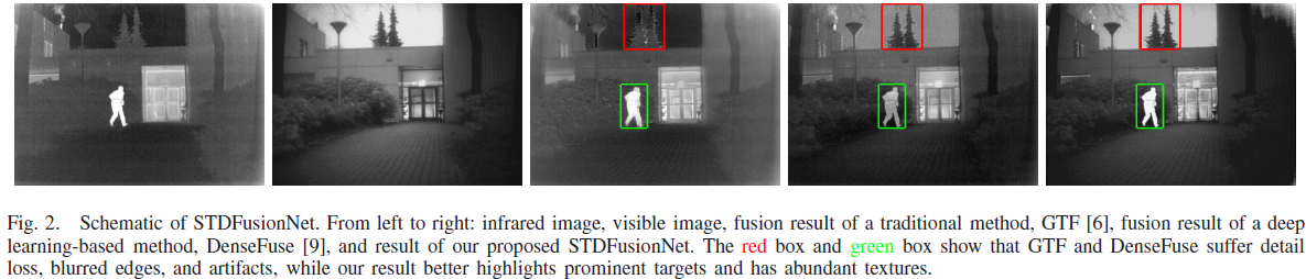
- 从左到右依次为红外、可见、传统方法GTF结果、深度方法DenseFuse结果、以及本文STDFusionNet结果;红框与绿框用于展示GTF与DenseFuse存在细节损失、边缘模糊、伪影,而STDFusionNet更好突出目标并具有丰富纹理。
3. 贡献
- 贡献1:定义融合过程中的“期望信息(desired information)”为红外图像的显著目标与可见图像的背景纹理的组合,并声称这是首次对红外-可见光融合目标的显式定义。
- 贡献2:将显著目标mask引入特定loss函数,引导网络检测红外热辐射目标并与可见背景纹理细节融合。
- 贡献3:大量实验显示该网络优越性;并指出融合结果“看起来像高质量可见光图像且目标突出”,有助于目标识别与场景理解。
4. 方法(STDFusionNet)
4.1 符号与“期望信息”定义
- 在红外-可见光融合中,最关键的信息是显著目标与纹理结构,分别来自红外图像与可见光图像;因此将“期望信息”显式定义为:红外图像中的显著目标信息 + 可见光图像中的背景纹理结构信息。
- 论文据此提出两项关键:
- 确定红外图像中的显著目标区域(通常是能发出更多热量的对象,如pedestrians/vehicles/bunkers所在区域);网络需要学习从红外图像中自动检测这些区域;
- 从检测到的区域准确提取期望信息并进行有效融合与重建,使融合结果在红外显著区域包含红外显著目标,在背景区域保留可见纹理。
- 在loss构建中,作者用显著目标mask 将“期望结果(desired result)”定义为:
其中 表示逐元素乘(element-wise multiplication)。
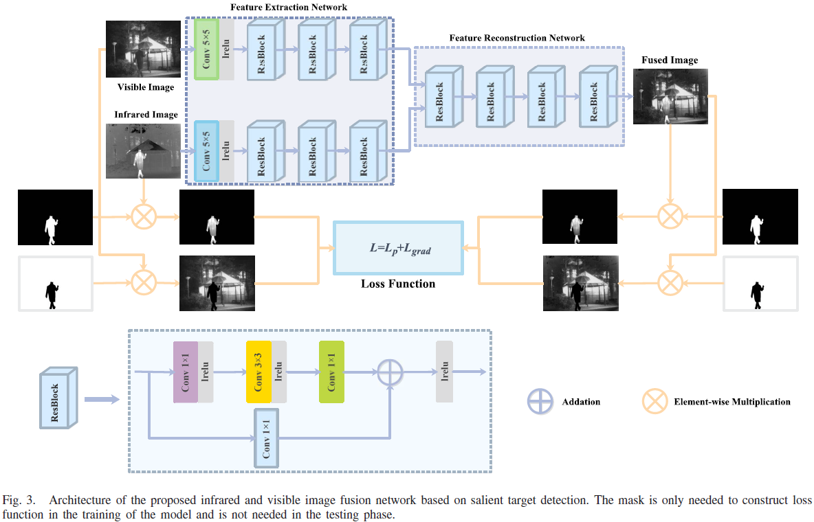
Fig.3:左侧的“Salient target mask”与其“背景mask(反相)”,在图中通过“逐元素乘”节点把源图像分成“显著区域”和“背景区域”。
4.2 总体框架
4.2.1 输入与“分区”操作(Fig.3左)
- 输入1:Visible Image(可见光图像),在Fig.3顶部作为可见分支的输入;同时在Fig.3下方参与与背景mask相乘以得到“可见背景区域”。
- 输入2:Infrared Image(红外图像),在Fig.3顶部作为红外分支的输入;同时在 Fig.3 下方参与与显著mask相乘以得到“红外显著区域”。
- 输入3:Salient target mask :此处说明其目的在于高亮红外图像中“能辐射大量热量”的对象(如 pedestrians/vehicles/bunkers)。
- 背景mask(Fig.3 中的反相mask):“salient target masks are inverted to obtain the background masks”。
- 逐像素乘(Fig.3 图例中的 element-wise multiplication):论文写到将显著mask与背景mask分别在像素级与红外/可见图像相乘,得到“source salient target regions”和“source background texture regions”。
对应实现:这部分是“mask分区”,属于训练期loss构建的前处理;并不意味着mask被送进主干网络作为输入。本文强调 mask仅用于训练期引导,不需要在测试期输入网络。
4.2.2 Feature Extraction Network(Fig.3顶部)
- 特征提取网络采用pseudosiamese架构以“区别对待”不同模态的源图像,从而选择性地从红外图像提取显著目标特征、从可见图像提取背景纹理特征。
- Fig.3顶部:可见分支与红外分支都先经过一个Conv 5×5和一个lrelu(leaky rectified linear unit),然后接 ResBlock×3。
- 该pseudosiamese架构中两条特征提取网络具有相同架构,但参数独立训练不共享,原因是红外与可见光图像属性不同。
4.2.3 Feature Reconstruction Network(Fig.3顶部右侧)
- Fig.3 中在两条特征提取分支之后进入Feature Reconstruction Network(虚线框部分),其内部由ResBlock×4组成,并最终输出融合图像 (“Fused Image”)。
- 特征重建网络的输入是红外卷积特征与可见卷积特征在通道维度上的拼接(concatenation in the channel dimension)。
- 重建网络最后一层使用Tanh激活,以保证输出图像取值范围与输入源图像一致。
4.2.4 Loss Function(Fig.3中部“Loss Function”块)
- Loss Function块中用简写表达了 “” 的思想;正文进一步说明其loss由两类损失构成:pixel loss(约束融合图像像素强度一致性)与gradient loss(促使融合图像包含更多细节信息)。
- 论文强调:pixel/gradient loss都分别在显著区域与背景区域构建,并结合显著mask 把融合图像划分为 (显著区域)与 (背景区域)。
4.3 Loss 公式(式(2)-(6))——像素一致 + 梯度一致 + 显著/背景分区
4.3.1 像素损失 Pixel loss(显著区域 / 背景区域)
- 显著区域像素损失:
- 背景区域像素损失:
- 论文说明: 为 L1 范数, 分别为图像高和宽。
4.3.2 梯度损失 Gradient loss(显著区域 / 背景区域)
- 论文写明:梯度算子 使用 Sobel operator 来计算图像梯度。
- 显著区域梯度损失:
- 背景区域梯度损失:
4.3.3 总损失——区域权重 + 同区域内 pixel/grad 等权
- 论文指出:与以往方法不同,作者在“同一个区域内”对 pixel loss 与 gradient loss 同等对待(equally),因此最终loss为:
- 论文解释: 是控制背景区域与显著区域 loss 平衡的权重;并指出通过在 loss 中引入显著区域约束,模型具有“自动检测并提取红外显著目标”的能力。
4.4 显著目标mask的获取与应用(Fig.3下半+Fig.4)
- 使用LabelMe toolbox标注红外图像中的显著目标并转成二值mask;之后将mask取反得到背景mask。
- 随后:
- 将显著mask与背景mask分别在像素级与红外/可见图像相乘,得到“源显著区域”和“源背景纹理区域”;
- 将融合图像同样与显著mask/背景mask相乘,得到“融合显著区域”和“融合背景区域”;
- 最终用这些区域去构造特定loss,从而引导网络隐式实现显著目标检测与信息融合。
- 显著目标mask仅用于训练引导,测试阶段不需要输入网络,因此模型端到端。
4.5 网络结构细节(Fig.3顶部/底部 ResBlock)
4.5.1 Feature Extraction Network(两条分支,pseudosiamese)
- 特征提取部分包含两条网络(红外/可见),二者架构相同但参数独立训练,以适应不同模态图像的属性差异。
- 每条特征提取网络由:
- Common layer:一个 5×5 卷积层 + 一个 leaky ReLU 激活层;
- 3 个 ResBlocks:用于增强提取的信息(“reinforce the extracted information”)。
4.5.2 ResBlock(Fig.3 底部局部结构:每一个点/算子)
- ResBlock 有两条路径:
主分支(上路):Conv1(1×1) → lrelu → Conv2(3×3) → lrelu → Conv3(1×1);
旁路(下路):identity conv(1×1)。
两路输出在“+”节点处相加后,再过一个 lrelu 输出。 - 除Conv2为 3×3 外,其余卷积核大小均为1×1;Conv1/Conv2后接 leaky ReLU;Conv3与identity conv输出先相加再接 leaky ReLU。
- identity conv的设计用于解决 ResBlock 输入与输出维度不一致的问题。
4.5.3 Feature Reconstruction Network(融合与重建)
- 特征重建网络由4个ResBlocks组成;其输入是红外与可见分支特征的通道拼接;最后一层使用Tanh激活以保证输出范围与输入一致。
4.5.4 padding/stride(“无下采样”)
- 信息丢失对融合任务是灾难性的,因此 STDFusionNet 的所有卷积层采用 padding = SAME 与 stride = 1;由此网络不引入下采样,融合图像尺寸与源图像一致。
5. 方法实现
按 Fig.3 + 式(1)-(6) 整理的训练/推理流程
数据预处理(归一化到 [-1,1]、裁剪 stride=24、patch=128×128;测试不裁剪)
来自 utils.input_setup 和 train.py。训练时每张源图/掩码都按 stride=24 滑窗裁成 128×128 patch,并用 (imread(...) - 127.5)/127.5 归一化到 [-1,1]。
def input_setup(sess, config, data_dir, index=0): """ Read image files and make their sub-images and saved them as a h5 file format. """ # Load data path if config.is_train: data = prepare_data(sess, dataset=data_dir) else: data = prepare_data(sess, dataset=data_dir)
sub_input_sequence = []
if config.is_train: for i in range(len(data)): input_ = (imread(data[i]) - 127.5) / 127.5 if len(input_.shape) == 3: h, w, _ = input_.shape else: h, w = input_.shape for x in range(0, h - config.image_size + 1, config.stride): for y in range(0, w - config.image_size + 1, config.stride): sub_input = input_[x:x + config.image_size, y:y + config.image_size] # Make channel value if data_dir == "Train": sub_input = cv2.resize(sub_input, (config.image_size / 4, config.image_size / 4), interpolation=cv2.INTER_CUBIC) sub_input = sub_input.reshape([config.image_size / 4, config.image_size / 4, 1]) print('error') else: sub_input = sub_input.reshape([config.image_size, config.image_size, 1])
sub_input_sequence.append(sub_input)
else: input_ = (imread(data[index]) - 127.5) / 127.5 // 归一化 if len(input_.shape) == 3: h_real, w_real, _ = input_.shape // RGB只关心HW else: h_real, w_real = input_.shape // IR只关心HW input_ = np.lib.pad(input_, ((padding, padding_h), (padding, padding_w)), 'edge') h, w = input_.shape # print(input_.shape) # Numbers of sub-images in height and width of image are needed to compute merge operation. nx = ny = 0 for x in range(0, h - config.image_size + 1, config.stride): nx += 1 ny = 0 for y in range(0, w - config.image_size + 1, config.stride): ny += 1 sub_input = input_[x:x + config.image_size, y:y + config.image_size] # [33 x 33] sub_input = sub_input.reshape([config.image_size, config.image_size, 1]) // 单通道输出,只关心亮度 sub_input_sequence.append(sub_input)// 128x128 每次64x64,右下,滑窗 """ len(sub_input_sequence) : the number of sub_input (33 x 33 x ch) in one image (sub_input_sequence[0]).shape : (33, 33, 1) """ # Make list to numpy array. With this transform arrdata = np.asarray(sub_input_sequence) # [?, 33, 33, 1] # print(arrdata.shape) make_data(sess, arrdata, data_dir)
if not config.is_train: print(nx, ny) print(h_real, w_real) return nx, ny, h_real, w_real- 对齐:
config.image_size=128、config.stride=24(见 5.5),对应训练细节“crop 128×128 with stride 24 得到 6921 patch”与“输入归一化到 [-1,1]”,且无下采样保持尺寸。 Train_vi、Train_ir、Train_ir_mask_blur通过该函数生成训练 patch,mask 仅进入 loss 计算(Fig.3 下半部分),测试阶段不需要 mask。
5.1 前向传播(Inference/Training都需要)
- 代码来源:
train_network.py。 - 包含两通路Visible Image与Infrared Image,和重建网络
class STDFusionNet(): def vi_feature_extraction_network(self, vi_image): // 这里定义的是可见光图像类 # 可见光编码器,输入 vi_image 形状: [N, H, W, 1] with tf.compat.v1.variable_scope('vi_extraction_network'): with tf.compat.v1.variable_scope('conv1'): # 首层 5x5 卷积提取低层特征,输出 16 通道 weights = tf.compat.v1.get_variable("w", [5, 5, 1, 16], initializer=tf.truncated_normal_initializer(stddev=1e-3)) #weights = weights_spectral_norm(weights) # 每个输出通道一个偏置 bias = tf.compat.v1.get_variable("b", [16], initializer=tf.constant_initializer(0.0)) # 步长 1 且 SAME 填充,保持空间尺寸 conv1 = tf.nn.conv2d(vi_image, weights, strides=[1, 1, 1, 1], padding='SAME') + bias # conv1 = tf.contrib.layers.batch_norm(conv1, decay=0.9, updates_collections=None, epsilon=1e-5, scale=True) # Leaky ReLU 激活缓解神经元死亡 conv1 = tf.nn.leaky_relu(conv1) block1_input = conv1 # state size: 16
// 主分支 1×1→3×3→1×1 且 Conv1/Conv2 后接 leaky ReLU,旁路 identity 1×1 升维;`conv3 + identity_conv` 后再过 leaky ReLU,对应 Fig.3 ResBlock 的“+”与激活。
with tf.compat.v1.variable_scope('block1'): with tf.compat.v1.variable_scope('conv1'): # 1x1 卷积混合通道,不改变空间分辨率 weights = tf.compat.v1.get_variable("w", [1, 1, 16, 16], initializer=tf.truncated_normal_initializer(stddev=1e-3)) #weights = weights_spectral_norm(weights) bias = tf.compat.v1.get_variable("b", [16], initializer=tf.constant_initializer(0.0)) # 点卷积投影 conv1 = tf.nn.conv2d(block1_input, weights, strides=[1, 1, 1, 1], padding='SAME') + bias conv1 = tf.nn.leaky_relu(conv1)
with tf.compat.v1.variable_scope('conv2'): # 3x3 卷积聚合空间上下文 weights = tf.compat.v1.get_variable("w", [3, 3, 16, 16], initializer=tf.truncated_normal_initializer(stddev=1e-3)) #weights = weights_spectral_norm(weights) bias = tf.compat.v1.get_variable("b", [16], initializer=tf.constant_initializer(0.0)) # SAME 填充保持特征图尺寸 conv2 = tf.nn.conv2d(conv1, weights, strides=[1, 1, 1, 1], padding='SAME') + bias conv2 = tf.nn.leaky_relu(conv2) with tf.compat.v1.variable_scope('conv3'): # 1x1 卷积生成残差输出 weights = tf.compat.v1.get_variable("w", [1, 1, 16, 16], initializer=tf.truncated_normal_initializer(stddev=1e-3)) #weights = weights_spectral_norm(weights) bias = tf.compat.v1.get_variable("b", [16], initializer=tf.constant_initializer(0.0)) # 残差分支输出 conv3 = tf.nn.conv2d(conv2, weights, strides=[1, 1, 1, 1], padding='SAME') + bias
# 残差连接:主分支与输入相加 block1_output = tf.nn.leaky_relu(conv3 + block1_input) block2_input = block1_output
with tf.compat.v1.variable_scope('block2'): with tf.compat.v1.variable_scope('conv1'): # 先用 1x1 通道混合,再做空间卷积 weights = tf.compat.v1.get_variable("w", [1, 1, 16, 16], initializer=tf.truncated_normal_initializer(stddev=1e-3)) #weights = weights_spectral_norm(weights) bias = tf.compat.v1.get_variable("b", [16], initializer=tf.constant_initializer(0.0)) # 点卷积投影 conv1 = tf.nn.conv2d(block2_input, weights, strides=[1, 1, 1, 1], padding='SAME') + bias conv1 = tf.nn.leaky_relu(conv1)
with tf.compat.v1.variable_scope('conv2'): # 3x3 卷积扩大感受野 weights = tf.compat.v1.get_variable("w", [3, 3, 16, 16], initializer=tf.truncated_normal_initializer(stddev=1e-3)) #weights = weights_spectral_norm(weights) bias = tf.compat.v1.get_variable("b", [16], initializer=tf.constant_initializer(0.0)) # SAME 填充保持分辨率 conv2 = tf.nn.conv2d(conv1, weights, strides=[1, 1, 1, 1], padding='SAME') + bias conv2 = tf.nn.leaky_relu(conv2) with tf.compat.v1.variable_scope('conv3'): # 1x1 卷积将通道升维到 32 weights = tf.compat.v1.get_variable("w", [1, 1, 16, 32], initializer=tf.truncated_normal_initializer(stddev=1e-3)) #weights = weights_spectral_norm(weights) bias = tf.compat.v1.get_variable("b", [32], initializer=tf.constant_initializer(0.0)) # 残差主分支输出 conv3 = tf.nn.conv2d(conv2, weights, strides=[1, 1, 1, 1], padding='SAME') + bias with tf.variable_scope('identity_conv'): # 投影捷径,将通道从 16 映射到 32 以便相加 weights = tf.compat.v1.get_variable("w", [1, 1, 16, 32], initializer=tf.truncated_normal_initializer(stddev=1e-3)) #weights = weights_spectral_norm(weights) identity_conv = tf.nn.conv2d(block2_input, weights, strides=[1, 1, 1, 1], padding='SAME') # 残差相加后再激活 block2_output = tf.nn.leaky_relu(conv3 + identity_conv) block3_input = block2_output
with tf.compat.v1.variable_scope('block3'): with tf.compat.v1.variable_scope('conv1'): # 1x1 通道混合,保持 32 通道 weights = tf.compat.v1.get_variable("w", [1, 1, 32, 32], initializer=tf.truncated_normal_initializer(stddev=1e-3)) #weights = weights_spectral_norm(weights) bias = tf.compat.v1.get_variable("b", [32], initializer=tf.constant_initializer(0.0)) # 点卷积投影 conv1 = tf.nn.conv2d(block3_input, weights, strides=[1, 1, 1, 1], padding='SAME') + bias conv1 = tf.nn.leaky_relu(conv1)
with tf.compat.v1.variable_scope('conv2'): # 3x3 卷积,通道仍为 32 weights = tf.compat.v1.get_variable("w", [3, 3, 32, 32], initializer=tf.truncated_normal_initializer(stddev=1e-3)) #weights = weights_spectral_norm(weights) bias = tf.compat.v1.get_variable("b", [32], initializer=tf.constant_initializer(0.0)) # SAME 填充的空间卷积 conv2 = tf.nn.conv2d(conv1, weights, strides=[1, 1, 1, 1], padding='SAME') + bias conv2 = tf.nn.leaky_relu(conv2) with tf.compat.v1.variable_scope('conv3'): # 1x1 卷积将通道升到 64 weights = tf.compat.v1.get_variable("w", [1, 1, 32, 64], initializer=tf.truncated_normal_initializer(stddev=1e-3)) #weights = weights_spectral_norm(weights) bias = tf.compat.v1.get_variable("b", [64], initializer=tf.constant_initializer(0.0)) # 残差主分支输出 conv3 = tf.nn.conv2d(conv2, weights, strides=[1, 1, 1, 1], padding='SAME') + bias with tf.variable_scope('identity_conv'): # 捷径分支投影,将 32 通道升到 64 weights = tf.compat.v1.get_variable("w", [1, 1, 32, 64], initializer=tf.truncated_normal_initializer(stddev=1e-3)) #weights = weights_spectral_norm(weights) identity_conv = tf.nn.conv2d(block3_input, weights, strides=[1, 1, 1, 1], padding='SAME') # 残差相加后的可见光编码输出 block3_output = tf.nn.leaky_relu(conv3 + identity_conv) encoding_feature = block3_output return encoding_feature
def ir_feature_extraction_network(self, ir_image): // 这里定义的是红外图像类 # 红外编码器,输入 ir_image 形状: [N, H, W, 1] with tf.compat.v1.variable_scope('ir_extraction_network'): with tf.compat.v1.variable_scope('conv1'): # 首层 5x5 卷积提取低层红外特征,输出 16 通道 weights = tf.compat.v1.get_variable("w", [5, 5, 1, 16], initializer=tf.truncated_normal_initializer(stddev=1e-3)) #weights = weights_spectral_norm(weights) # 每通道偏置 bias = tf.compat.v1.get_variable("b", [16], initializer=tf.constant_initializer(0.0)) # SAME 填充保持尺寸,步长 1 conv1 = tf.nn.conv2d(ir_image, weights, strides=[1, 1, 1, 1], padding='SAME') + bias # conv1 = tf.contrib.layers.batch_norm(conv1, decay=0.9, updates_collections=None, epsilon=1e-5, scale=True) # Leaky ReLU 激活 conv1 = tf.nn.leaky_relu(conv1) block1_input = conv1 # state size: 16
// 主分支 1×1→3×3→1×1 且 Conv1/Conv2 后接 leaky ReLU,旁路 identity 1×1 升维;`conv3 + identity_conv` 后再过 leaky ReLU,对应 Fig.3 ResBlock 的“+”与激活。
with tf.compat.v1.variable_scope('block1'): with tf.compat.v1.variable_scope('conv1'): # 1x1 通道混合,保持空间 weights = tf.compat.v1.get_variable("w", [1, 1, 16, 16], initializer=tf.truncated_normal_initializer(stddev=1e-3)) #weights = weights_spectral_norm(weights) bias = tf.compat.v1.get_variable("b", [16], initializer=tf.constant_initializer(0.0)) # 点卷积投影 conv1 = tf.nn.conv2d(block1_input, weights, strides=[1, 1, 1, 1], padding='SAME') + bias conv1 = tf.nn.leaky_relu(conv1)
with tf.compat.v1.variable_scope('conv2'): # 3x3 卷积获取局部上下文 weights = tf.compat.v1.get_variable("w", [3, 3, 16, 16], initializer=tf.truncated_normal_initializer(stddev=1e-3)) #weights = weights_spectral_norm(weights) bias = tf.compat.v1.get_variable("b", [16], initializer=tf.constant_initializer(0.0)) # SAME 填充,步长 1 conv2 = tf.nn.conv2d(conv1, weights, strides=[1, 1, 1, 1], padding='SAME') + bias conv2 = tf.nn.leaky_relu(conv2) with tf.compat.v1.variable_scope('conv3'): # 1x1 卷积生成残差输出(仍 16 通道) weights = tf.compat.v1.get_variable("w", [1, 1, 16, 16], initializer=tf.truncated_normal_initializer(stddev=1e-3)) #weights = weights_spectral_norm(weights) bias = tf.compat.v1.get_variable("b", [16], initializer=tf.constant_initializer(0.0)) # 残差主分支输出 conv3 = tf.nn.conv2d(conv2, weights, strides=[1, 1, 1, 1], padding='SAME') + bias
# 残差连接:与输入相加再激活 block1_output = tf.nn.leaky_relu(conv3 + block1_input) block2_input = block1_output
with tf.compat.v1.variable_scope('block2'): with tf.compat.v1.variable_scope('conv1'): # 1x1 通道混合,为升维做准备 weights = tf.compat.v1.get_variable("w", [1, 1, 16, 16], initializer=tf.truncated_normal_initializer(stddev=1e-3)) #weights = weights_spectral_norm(weights) bias = tf.compat.v1.get_variable("b", [16], initializer=tf.constant_initializer(0.0)) # 点卷积投影 conv1 = tf.nn.conv2d(block2_input, weights, strides=[1, 1, 1, 1], padding='SAME') + bias conv1 = tf.nn.leaky_relu(conv1)
with tf.compat.v1.variable_scope('conv2'): # 3x3 卷积扩大感受野 weights = tf.compat.v1.get_variable("w", [3, 3, 16, 16], initializer=tf.truncated_normal_initializer(stddev=1e-3)) #weights = weights_spectral_norm(weights) bias = tf.compat.v1.get_variable("b", [16], initializer=tf.constant_initializer(0.0)) # SAME 填充保持尺寸 conv2 = tf.nn.conv2d(conv1, weights, strides=[1, 1, 1, 1], padding='SAME') + bias conv2 = tf.nn.leaky_relu(conv2) with tf.compat.v1.variable_scope('conv3'): # 1x1 卷积升维至 32 通道 weights = tf.compat.v1.get_variable("w", [1, 1, 16, 32], initializer=tf.truncated_normal_initializer(stddev=1e-3)) #weights = weights_spectral_norm(weights) bias = tf.compat.v1.get_variable("b", [32], initializer=tf.constant_initializer(0.0)) # 残差主分支输出 conv3 = tf.nn.conv2d(conv2, weights, strides=[1, 1, 1, 1], padding='SAME') + bias with tf.variable_scope('identity_conv'): # 捷径投影,将 16 通道映射到 32 通道 weights = tf.compat.v1.get_variable("w", [1, 1, 16, 32], initializer=tf.truncated_normal_initializer(stddev=1e-3)) #weights = weights_spectral_norm(weights) identity_conv = tf.nn.conv2d(block2_input, weights, strides=[1, 1, 1, 1], padding='SAME') # 残差相加并激活 block2_output = tf.nn.leaky_relu(conv3 + identity_conv) block3_input = block2_output
with tf.compat.v1.variable_scope('block3'): with tf.compat.v1.variable_scope('conv1'): # 1x1 通道混合,保持 32 通道 weights = tf.compat.v1.get_variable("w", [1, 1, 32, 32], initializer=tf.truncated_normal_initializer(stddev=1e-3)) #weights = weights_spectral_norm(weights) bias = tf.compat.v1.get_variable("b", [32], initializer=tf.constant_initializer(0.0)) # 点卷积投影 conv1 = tf.nn.conv2d(block3_input, weights, strides=[1, 1, 1, 1], padding='SAME') + bias conv1 = tf.nn.leaky_relu(conv1)
with tf.compat.v1.variable_scope('conv2'): # 3x3 卷积保持 32 通道 weights = tf.compat.v1.get_variable("w", [3, 3, 32, 32], initializer=tf.truncated_normal_initializer(stddev=1e-3)) #weights = weights_spectral_norm(weights) bias = tf.compat.v1.get_variable("b", [32], initializer=tf.constant_initializer(0.0)) # SAME 填充卷积 conv2 = tf.nn.conv2d(conv1, weights, strides=[1, 1, 1, 1], padding='SAME') + bias conv2 = tf.nn.leaky_relu(conv2) with tf.compat.v1.variable_scope('conv3'): # 1x1 卷积升维到 64 通道 weights = tf.compat.v1.get_variable("w", [1, 1, 32, 64], initializer=tf.truncated_normal_initializer(stddev=1e-3)) #weights = weights_spectral_norm(weights) bias = tf.compat.v1.get_variable("b", [64], initializer=tf.constant_initializer(0.0)) # 残差主分支输出 conv3 = tf.nn.conv2d(conv2, weights, strides=[1, 1, 1, 1], padding='SAME') + bias with tf.variable_scope('identity_conv'): # 捷径分支投影,32 -> 64 通道 weights = tf.compat.v1.get_variable("w", [1, 1, 32, 64], initializer=tf.truncated_normal_initializer(stddev=1e-3)) #weights = weights_spectral_norm(weights) identity_conv = tf.nn.conv2d(block3_input, weights, strides=[1, 1, 1, 1], padding='SAME') # 残差输出,得到红外编码特征 block3_output = tf.nn.leaky_relu(conv3 + identity_conv) encoding_feature = block3_output return encoding_feature
def feature_reconstruction_network(self, feature): // decoder重建网络 # 解码重建网络,将拼接特征还原为融合图像 with tf.compat.v1.variable_scope('reconstruction_network'): block1_input = feature with tf.compat.v1.variable_scope('block1'): with tf.compat.v1.variable_scope('conv1'): # 1x1 通道混合,保持 128 通道 weights = tf.compat.v1.get_variable("w", [1, 1, 128, 128], initializer=tf.truncated_normal_initializer(stddev=1e-3)) #weights = weights_spectral_norm(weights) bias = tf.compat.v1.get_variable("b", [128], initializer=tf.constant_initializer(0.0)) # 点卷积 conv1 = tf.nn.conv2d(block1_input, weights, strides=[1, 1, 1, 1], padding='SAME') + bias conv1 = tf.nn.leaky_relu(conv1)
with tf.compat.v1.variable_scope('conv2'): # 3x3 卷积保持通道,提炼空间信息 weights = tf.compat.v1.get_variable("w", [3, 3, 128, 128], initializer=tf.truncated_normal_initializer(stddev=1e-3)) #weights = weights_spectral_norm(weights) bias = tf.compat.v1.get_variable("b", [128], initializer=tf.constant_initializer(0.0)) # SAME 填充卷积 conv2 = tf.nn.conv2d(conv1, weights, strides=[1, 1, 1, 1], padding='SAME') + bias conv2 = tf.nn.leaky_relu(conv2) with tf.compat.v1.variable_scope('conv3'): # 1x1 卷积降维至 64 通道 weights = tf.compat.v1.get_variable("w", [1, 1, 128, 64], initializer=tf.truncated_normal_initializer(stddev=1e-3)) #weights = weights_spectral_norm(weights) bias = tf.compat.v1.get_variable("b", [64], initializer=tf.constant_initializer(0.0)) # 残差主分支输出 conv3 = tf.nn.conv2d(conv2, weights, strides=[1, 1, 1, 1], padding='SAME') + bias with tf.variable_scope('identity_conv'): # 捷径投影 128 -> 64,匹配相加 weights = tf.compat.v1.get_variable("w", [1, 1, 128, 64], initializer=tf.truncated_normal_initializer(stddev=1e-3)) #weights = weights_spectral_norm(weights) identity_conv = tf.nn.conv2d(block1_input, weights, strides=[1, 1, 1, 1], padding='SAME') # 残差相加,使用 ELU 稳定梯度 block1_output = tf.nn.elu(conv3 + identity_conv) block2_input = block1_output with tf.compat.v1.variable_scope('block2'): with tf.compat.v1.variable_scope('conv1'): # 1x1 通道混合,维持 64 通道 weights = tf.compat.v1.get_variable("w", [1, 1, 64, 64], initializer=tf.truncated_normal_initializer(stddev=1e-3)) #weights = weights_spectral_norm(weights) bias = tf.compat.v1.get_variable("b", [64], initializer=tf.constant_initializer(0.0)) # 点卷积 conv1 = tf.nn.conv2d(block2_input, weights, strides=[1, 1, 1, 1], padding='SAME') + bias conv1 = tf.nn.leaky_relu(conv1)
with tf.compat.v1.variable_scope('conv2'): # 3x3 卷积保持 64 通道 weights = tf.compat.v1.get_variable("w", [3, 3, 64, 64], initializer=tf.truncated_normal_initializer(stddev=1e-3)) #weights = weights_spectral_norm(weights) bias = tf.compat.v1.get_variable("b", [64], initializer=tf.constant_initializer(0.0)) # SAME 卷积 conv2 = tf.nn.conv2d(conv1, weights, strides=[1, 1, 1, 1], padding='SAME') + bias conv2 = tf.nn.leaky_relu(conv2) with tf.compat.v1.variable_scope('conv3'): # 1x1 卷积降维到 32 通道 weights = tf.compat.v1.get_variable("w", [1, 1, 64, 32], initializer=tf.truncated_normal_initializer(stddev=1e-3)) #weights = weights_spectral_norm(weights) bias = tf.compat.v1.get_variable("b", [32], initializer=tf.constant_initializer(0.0)) # 残差主分支 conv3 = tf.nn.conv2d(conv2, weights, strides=[1, 1, 1, 1], padding='SAME') + bias with tf.variable_scope('identity_conv'): # 捷径投影 64 -> 32 weights = tf.compat.v1.get_variable("w", [1, 1, 64, 32], initializer=tf.truncated_normal_initializer(stddev=1e-3)) #weights = weights_spectral_norm(weights) identity_conv = tf.nn.conv2d(block2_input, weights, strides=[1, 1, 1, 1], padding='SAME') # 残差相加再 ELU 激活 block2_output = tf.nn.elu(conv3 + identity_conv) block3_input = block2_output with tf.compat.v1.variable_scope('block3'): with tf.compat.v1.variable_scope('conv1'): # 1x1 卷积保持 32 通道 weights = tf.compat.v1.get_variable("w", [1, 1, 32, 32], initializer=tf.truncated_normal_initializer(stddev=1e-3)) #weights = weights_spectral_norm(weights) bias = tf.compat.v1.get_variable("b", [32], initializer=tf.constant_initializer(0.0)) # 点卷积 conv1 = tf.nn.conv2d(block3_input, weights, strides=[1, 1, 1, 1], padding='SAME') + bias conv1 = tf.nn.leaky_relu(conv1)
with tf.compat.v1.variable_scope('conv2'): # 3x3 卷积保持 32 通道 weights = tf.compat.v1.get_variable("w", [3, 3, 32, 32], initializer=tf.truncated_normal_initializer(stddev=1e-3)) #weights = weights_spectral_norm(weights) bias = tf.compat.v1.get_variable("b", [32], initializer=tf.constant_initializer(0.0)) # SAME 卷积 conv2 = tf.nn.conv2d(conv1, weights, strides=[1, 1, 1, 1], padding='SAME') + bias conv2 = tf.nn.leaky_relu(conv2) with tf.compat.v1.variable_scope('conv3'): # 1x1 卷积降到 16 通道 weights = tf.compat.v1.get_variable("w", [1, 1, 32, 16], initializer=tf.truncated_normal_initializer(stddev=1e-3)) #weights = weights_spectral_norm(weights) bias = tf.compat.v1.get_variable("b", [16], initializer=tf.constant_initializer(0.0)) # 残差主分支 conv3 = tf.nn.conv2d(conv2, weights, strides=[1, 1, 1, 1], padding='SAME') + bias with tf.variable_scope('identity_conv'): # 捷径投影 32 -> 16 weights = tf.compat.v1.get_variable("w", [1, 1, 32, 16], initializer=tf.truncated_normal_initializer(stddev=1e-3)) #weights = weights_spectral_norm(weights) identity_conv = tf.nn.conv2d(block3_input, weights, strides=[1, 1, 1, 1], padding='SAME') # 残差相加后激活 block3_output = tf.nn.leaky_relu(conv3 + identity_conv) block4_input = block3_output with tf.compat.v1.variable_scope('block4'): with tf.compat.v1.variable_scope('conv1'): # 1x1 卷积保持 16 通道 weights = tf.compat.v1.get_variable("w", [1, 1, 16, 16], initializer=tf.truncated_normal_initializer(stddev=1e-3)) #weights = weights_spectral_norm(weights) bias = tf.compat.v1.get_variable("b", [16], initializer=tf.constant_initializer(0.0)) # 点卷积 conv1 = tf.nn.conv2d(block4_input, weights, strides=[1, 1, 1, 1], padding='SAME') + bias conv1 = tf.nn.leaky_relu(conv1)
with tf.compat.v1.variable_scope('conv2'): # 3x3 卷积保持 16 通道 weights = tf.compat.v1.get_variable("w", [3, 3, 16, 16], initializer=tf.truncated_normal_initializer(stddev=1e-3)) #weights = weights_spectral_norm(weights) bias = tf.compat.v1.get_variable("b", [16], initializer=tf.constant_initializer(0.0)) # SAME 卷积 conv2 = tf.nn.conv2d(conv1, weights, strides=[1, 1, 1, 1], padding='SAME') + bias conv2 = tf.nn.leaky_relu(conv2) with tf.compat.v1.variable_scope('conv3'): # 1x1 卷积生成单通道输出 weights = tf.compat.v1.get_variable("w", [1, 1, 16, 1], initializer=tf.truncated_normal_initializer(stddev=1e-3)) #weights = weights_spectral_norm(weights) bias = tf.compat.v1.get_variable("b", [1], initializer=tf.constant_initializer(0.0)) # 残差主分支输出 conv3 = tf.nn.conv2d(conv2, weights, strides=[1, 1, 1, 1], padding='SAME') + bias with tf.variable_scope('identity_conv'): # 捷径分支保持 1 通道,便于相加 weights = tf.compat.v1.get_variable("w", [1, 1, 16, 1], initializer=tf.truncated_normal_initializer(stddev=1e-3)) #weights = weights_spectral_norm(weights) identity_conv = tf.nn.conv2d(block4_input, weights, strides=[1, 1, 1, 1], padding='SAME') # 残差相加后用 tanh 输出融合图像 block4_output = tf.nn.tanh(conv3 + identity_conv) fusion_image = block4_output return fusion_image def STDFusion_model(self, vi_image, ir_image): # 整体模型:编码可见光与红外,拼接后解码得到融合图像 with tf.variable_scope("STDFusion_model"): # 提取可见光特征 vi_feature = self.vi_feature_extraction_network(vi_image) # 提取红外特征 ir_feature = self.ir_feature_extraction_network(ir_image) # 通道维拼接形成联合特征 feature = tf.concat([vi_feature, ir_feature], axis=-1) # 解码重建融合图像 f_image = self.feature_reconstruction_network(feature) return f_image5.2 Sobel 梯度算子(对应式(4)(5)中的 ∇)
def gradient(input): filter1 = tf.reshape(tf.constant([[-1., 0., 1.], [-2., 0., 2.], [-1., 0., 1.]]), [3, 3, 1, 1]) filter2 = tf.reshape(tf.constant([[-1., -2., -1.], [0., 0., 0.], [1., 2., 1.]]), [3, 3, 1, 1]) Gradient1 = tf.nn.conv2d(input, filter1, strides=[1, 1, 1, 1], padding='SAME') Gradient2 = tf.nn.conv2d(input, filter2, strides=[1, 1, 1, 1], padding='SAME') Gradient = tf.abs(Gradient1) + tf.abs(Gradient2) return Gradient- 代码来源:
utils.py。 filter1/2为 Sobel 水平/垂直核,对应原文中“we employ the Sobel operator”;输出Gradient即式(4)(5) 中的 。
5.3 Loss 计算(对应式(2)-(6),含 mask 分区)
with tf.name_scope('g_loss'): self.ir_mask = (self.ir_mask + 1) / 2.0 self.ir_p_loss_train = tf.multiply(self.ir_mask, tf.abs(self.fusion_images - self.ir_images)) self.vi_p_loss_train = tf.multiply(1 - self.ir_mask, tf.abs(self.fusion_images - self.vi_images)) self.ir_grad_loss_train = tf.multiply(self.ir_mask, tf.abs(gradient(self.fusion_images) - gradient(self.ir_images))) self.vi_grad_loss_train = tf.multiply(1 - self.ir_mask, tf.abs(gradient(self.fusion_images) - gradient(self.vi_images)))
self.ir_p_loss = tf.reduce_mean(self.ir_p_loss_train) self.vi_p_loss = tf.reduce_mean(self.vi_p_loss_train) self.ir_grad_loss = tf.reduce_mean(self.ir_grad_loss_train) self.vi_grad_loss = tf.reduce_mean(self.vi_grad_loss_train) self.g_loss_2 = 1 * self.vi_p_loss + 1 * self.vi_grad_loss + 7 * self.ir_p_loss + 7 * self.ir_grad_loss- 代码来源:
model.py。 (mask+1)/2恢复二值显著区域;1 - ir_mask是背景 mask(“inverted”);四项对应式(2)–(5) 的显著/背景像素与梯度 L1,reduce_mean实现 。g_loss_2中显著区域乘 ,背景系数为 1,对应式(6)。
5.4 训练流程(“Training Details”)
flags.DEFINE_integer("epoch", 30, "Number of epoch [10]")flags.DEFINE_integer("batch_size", 32, "The size of batch images [128]")flags.DEFINE_integer("image_size", 128, "The size of image to use [33]")flags.DEFINE_integer("stride", 24, "The size of stride to apply input image [14]")flags.DEFINE_float("learning_rate", 1e-3, "The learning rate of gradient descent algorithm [1e-4]")with tf.name_scope('train_step'): self.train_generator_op = tf.train.AdamOptimizer(config.learning_rate).minimize(self.g_loss_total, var_list=self.g_vars)for ep in range(config.epoch): lr = self.init_lr if ep < self.decay_epoch else self.init_lr * (config.epoch - ep) / (config.epoch - self.decay_epoch) batch_idxs = len(train_data_ir) // config.batch_size for idx in range(0, batch_idxs): batch_vi_images = train_data_vi[idx * config.batch_size: (idx + 1) * config.batch_size] batch_ir_images = train_data_ir[idx * config.batch_size: (idx + 1) * config.batch_size] batch_ir_mask = train_data_ir_mask[idx * config.batch_size: (idx + 1) * config.batch_size] batch_ir_mask = (batch_ir_mask + 1.0) / 2.0 _, err_g, batch_vi_p_loss, batch_ir_p_loss, batch_vi_grad_loss, batch_ir_grad_loss, summary_str = self.sess.run( [self.train_generator_op, self.g_loss_total, self.vi_p_loss, self.ir_p_loss, self.vi_grad_loss, self.ir_grad_loss, self.summary_op], feed_dict={self.vi_images: batch_vi_images, self.ir_images: batch_ir_images, self.ir_mask: batch_ir_mask, self.lr: lr})- 代码来源:
train.py(超参)与model.py(训练循环)。 epoch=30、batch_size=32、learning_rate=1e-3、stride=24、image_size=128完全对齐原论文训练设置;Adam 优化器即原文“TensorFlow + Adam”。训练集为 TNO 20 对图像,经 5.1 裁剪共 6921 对 patch;测试阶段不裁剪且不输入 mask。
6. 实验设置(Datasets / Metrics / Training Details)
6.1 数据集(TNO & RoadScene)
- 论文在实验中使用两个数据集:TNO 与 RoadScene。
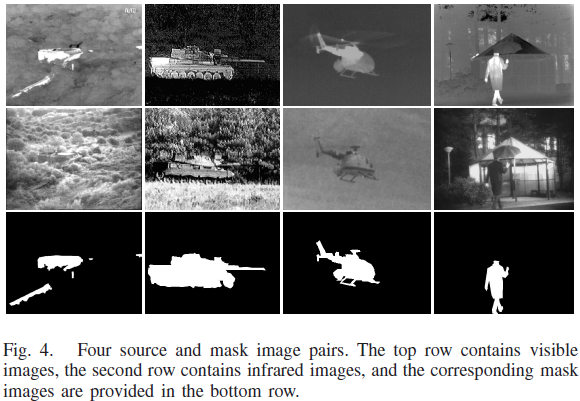
- TNO:包含 60 对红外/可见图像,分为三个序列,分别含 19、23、32 对;Fig.4 给出典型源图像与对应mask示例。
- RoadScene:由 Xu 等基于 FLIR 视频发布,包含 221 对对齐的红外/可见图像,场景包含道路、车辆、行人,并被描述为缓解“样本少与低分辨率”的挑战。
6.2 指标(EN / MI / VIF / SF)
- 论文选择四个常用指标:EN、MI、VIF、SF,并在文中给出其定义公式;并说明客观评价是对主观评价的补充。
- 论文给出 SF 的定义并指出:SF 大意味着融合图像含有更丰富的纹理与细节,从而性能更好。
6.3 训练细节(Training Details)
- 训练:在 TNO 上训练,训练图像对数量为 20;为获得更多数据,设置 stride=24 进行裁剪,每个 patch 大小 128×128,得到 6921 对 patch。
- 测试:在 TNO 选 20 对做对比实验,在 RoadScene 选 20 对做泛化实验;并强调测试时源图像直接输入网络、不做裁剪。
- 归一化与优化:源图像归一化到 [-1,1];使用 Adam;实现平台 TensorFlow;batch size=32,iteration=30,学习率 1e-3。
- 取值:论文观察到显著区域只占红外图像很小比例,因此为平衡显著/背景区域的loss,设 。硬件:NVIDIA TITAN V GPU + 2.00-GHz Intel Xeon Gold 5117 CPU。
7. 对比实验结果
7.1 对比方法(9个)
- 论文比较9种方法:传统方法 GTF、MDLatLRR;深度方法 DenseFuse、NestFuse、FusionGAN、GANMcC、IFCNN、PMGI、U2Fusion,并说明这些方法实现公开且参数按原文设置。
7.2 TNO:主观结果(Figs.5–8)与论文给出的观察
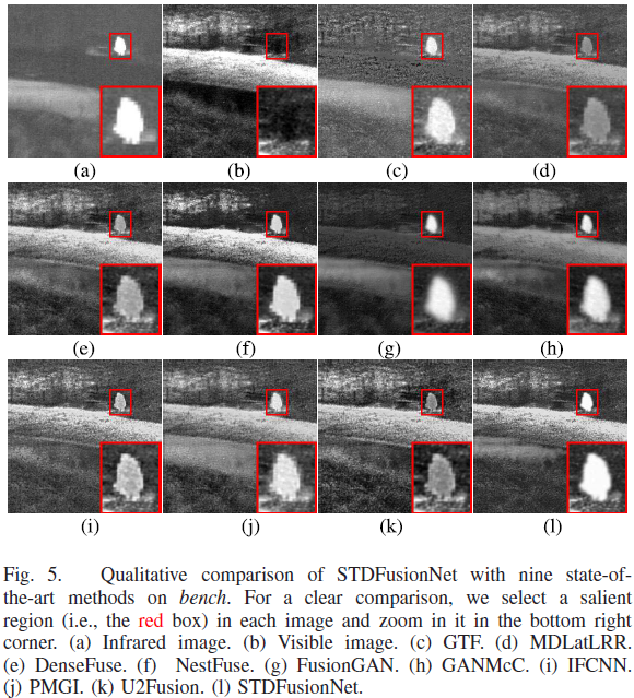
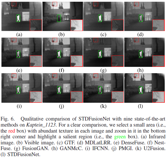
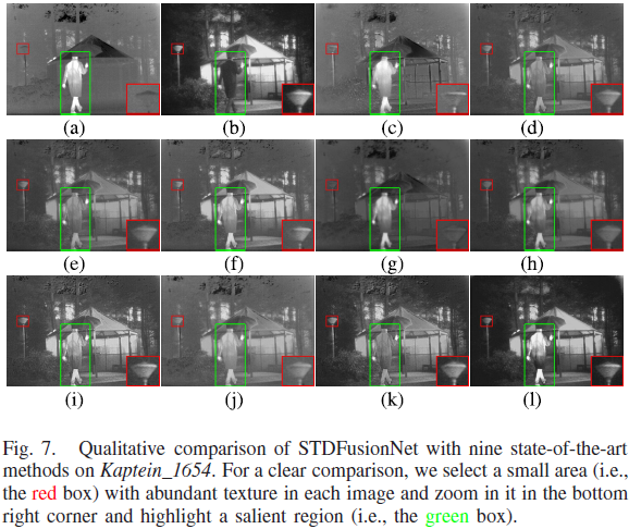
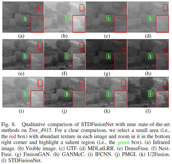
- 论文在 TNO 上选择四个典型图像对(bench、Kaptein_1123、Kaptein_1654、Tree_4915)做主观评价,并在 Fig.5 中用红框标注显著区域进行放大对比。
- 论文描述(Fig.5):MDLatLRR 会丢失热辐射目标信息;DenseFuse/IFCNN/U2Fusion 虽保留热辐射目标信息,但受到严重噪声污染(来源为可见图像信息)。
- 论文总结四个场景:STDFusionNet 不仅能有效突出显著目标,还在保持背景纹理细节方面有明显优势;并举例说明:Kaptein_1123 中树枝纹理最清晰且天空不被热辐射污染;Kaptein_1654 中背景路灯与可见图几乎一致;Tree_4915 中其他方法几乎无法区分灌木与背景,而 STDFusionNet 能突出红外目标并区分灌木。
- 论文指出:这种“选择性保留红外显著目标 + 可见纹理细节”的表现,主要得益于训练时人工提取的显著目标mask与构造的loss函数。
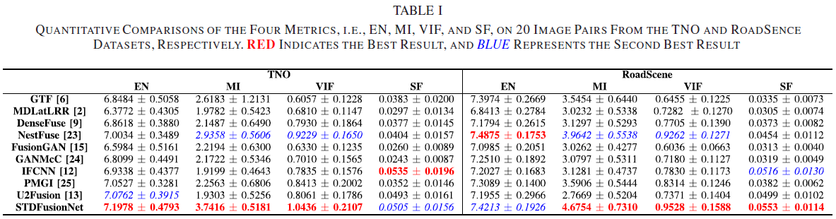
7.3 TNO:客观结果(Fig.9 + Table I)与论文对指标的解释
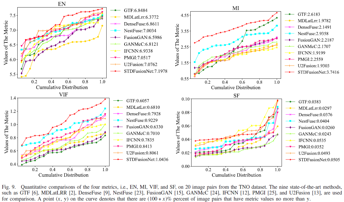
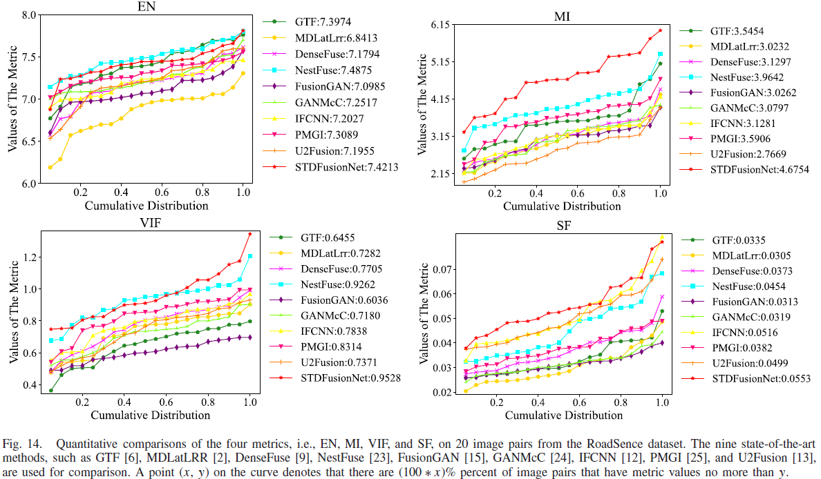
- Fig.9 的题注说明:在 TNO 的 20 对图像上对 EN/MI/VIF/SF 做曲线对比;曲线上一点 (x,y) 表示有 (100*x)% 的图像对的指标值不超过 y;并列出用于比较的9种方法名称。
- 论文对 TNO 的定量结论:在四个指标中,STDFusionNet 在 EN、MI、VIF 三项上优势显著;SF 指标仅以很小差距落后于 IFCNN。
- 论文强调:STDFusionNet 在 VIF 上几乎所有图像对都取最高值,这与主观评价一致,表明其融合图像具有更好的视觉效果;并解释 EN 最大说明信息更丰富、MI 最大说明从源图像传递的信息更多;SF 虽非最佳但“可比结果”表明融合结果具备足够梯度信息。
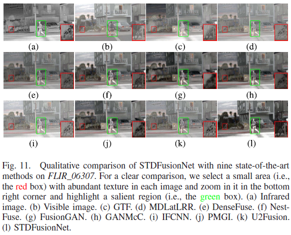
7.4 泛化实验(RoadScene):彩色可见图像的融合策略 + 论文观察
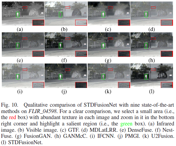
- 泛化设置:使用 RoadScene 测试在 TNO 上训练的模型,以评估泛化能力。
- 因 RoadScene 可见图像为彩色,论文采用特定融合策略以保色:RGB→YCbCr;将 Y 通道与灰度红外图像进行融合;再用可见图的 Cb/Cr 做逆变换恢复 RGB 融合结果。
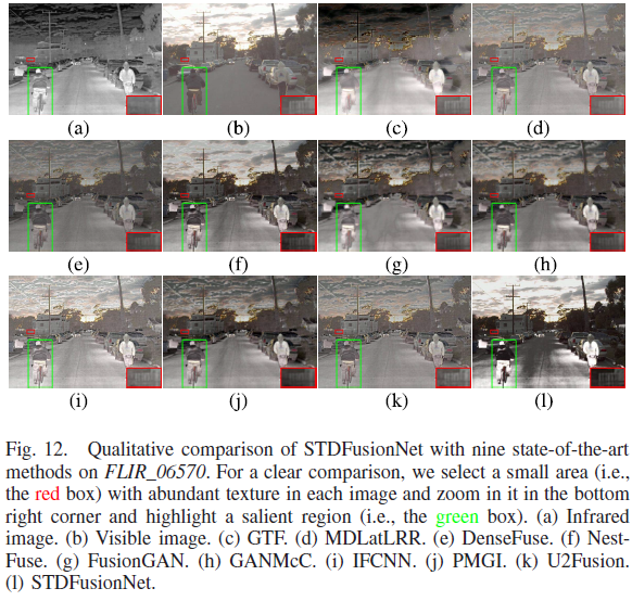
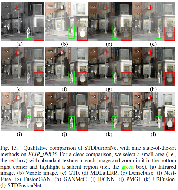
- 论文对 Figs.10–13 的观察:STDFusionNet 能选择性保留红外与可见的有用信息;其融合图像在显著区域非常接近红外图像,且背景区域几乎完整保留可见纹理结构;而其他方法虽然能突出目标,但融合背景“极不令人满意”,例如天空被热信息严重污染,影响对时间/天气判断;同时其他方法对墙面文字、车辆、树桩、栅栏、路灯等背景细节保留不佳,STDFusionNet 则能有效保留背景细节并维持/增强目标对比度。
- 论文对 RoadScene 的定量结论:STDFusionNet 在 MI/VIF/SF 的平均值最好;EN 指标仅以很小差距落后 NestFuse;并据此认为其具有良好泛化性,受成像传感器特性影响较小。
7.5 效率对比(Table II)与论文结论
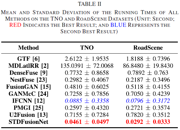
- 论文指出:运行效率也是重要因素;Table II 给出在 TNO 与 RoadScene 上不同方法的平均运行时间;并指出深度方法因 GPU 加速在运行时间上有优势,尤其是 STDFusionNet;传统方法耗时更长,MDLatLRR 因分解过程尤其耗时。
- 论文结论:STDFusionNet 在两数据集上具有最小平均运行时间与最小标准差,说明网络对不同分辨率源图像具有鲁棒性并证明了结构设计的效率。
8. “显著目标检测”可视化(Fig.15)
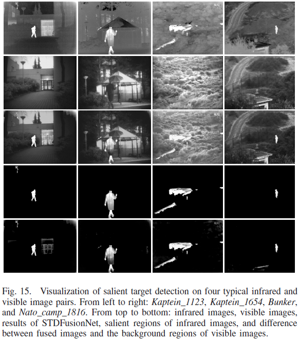
- 论文写到:STDFusionNet 可“隐式”实现显著目标检测,并给出可视化:展示红外图像的显著区域,以及“从融合结果中减去可见背景区域”的差分结果。
- 论文指出:差分结果与红外显著区域基本一致,且存在“额外的热显著目标”被方法检测到的现象,从而表明 STDFusionNet 能隐式执行显著目标检测。
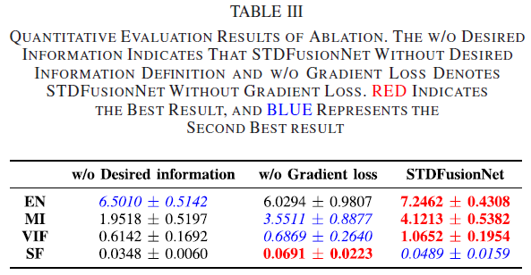
9. 消融实验(Fig.16 + Table III):期望信息定义 & 梯度loss
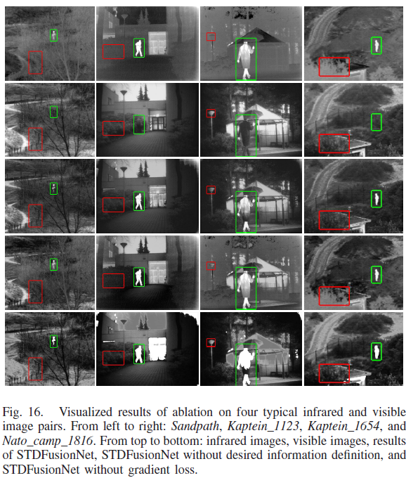
9.1 w/o desired information(去掉“期望信息定义”的消融)
- 为验证“期望信息定义”的合理性,在 TNO 上训练两种模型,主要差异是是否将显著目标mask引入loss;当移除显著mask后,不需要区分显著/背景区域,因此将 设为 1。
- 论文在 Fig.16 中描述:有期望信息定义时,STDFusionNet 的结果能突出显著目标并维持背景纹理;不使用期望信息定义时,网络以“coarse manner”进行融合,导致显著区域的热辐射信息与背景纹理信息都不能很好保留。
9.2 w/o gradient loss(去掉梯度loss的消融)
- 论文在 Fig.16 附近写到:移除 gradient loss 时,显著区域几乎没有纹理信息,显著目标形状出现严重扭曲,背景区域也出现伪影;并且在 Table III 中除 SF 外其他指标呈下降趋势,论文据此强调 gradient loss 的重要性:它能确保融合图像中显著目标的纹理清晰度(texture sharpness)。
10. 结论(Conclusion)
- 提出 STDFusionNet,并将红外-可见光融合的期望信息显式定义为“红外显著区域 + 可见背景区域”;在此基础上把显著目标mask引入loss以精确引导网络优化。
- 模型可隐式完成显著目标检测与信息融合,融合结果既包含显著热目标也具有丰富背景纹理;大量主观与客观实验验证其优越性,并且运行速度更快。
文章分享
如果这篇文章对你有帮助,欢迎分享给更多人!
【论文阅读 | TIM 2021 | STDFusionNet:基于显著目标检测的红外-可见光图像融合网络】
https://mjy.js.org/posts/论文阅读--tim-2021--stdfusionnet基于显著目标检测的红外-可见光图像融合网络/