Pytorch教程 搭建一个神经网络
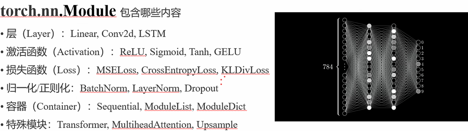
PyTorch 常用层讲解与示例 本教程介绍 PyTorch 中一些核心神经网络层:Linear、Conv2d、LSTM,包括它们的数学公式和对应实现代码。
1. Linear 层 (全连接层) 数学公式 :
输入向量 x ∈ R d i n x \in \mathbb{R}^{d_{in}} x ∈ R d in y ∈ R d o u t y \in \mathbb{R}^{d_{out}} y ∈ R d o u t
y = x W ⊤ + b , W ∈ R d o u t × d i n , b ∈ R d o u t y = x W^\top + b, \quad W \in \mathbb{R}^{d_{out} \times d_{in}}, \quad b \in \mathbb{R}^{d_{out}} y = x W ⊤ + b , W ∈ R d o u t × d in , b ∈ R d o u t 解释 :
每个输出节点是输入节点的加权和加上偏置 常用于全连接网络、MLP 等 示例代码 :
1
2
3
4
5
6
7
8
9
10
11
12
13
14
15
16
17
import torchimport torch.nn as nnclass LinearExample (nn.Module): def __init__ (self, d_in, d_out ): super ().__init__() self .linear = nn.Linear(d_in, d_out) def forward (self, x ): return self .linear(x) x = torch.randn(4 , 10 ) model_linear = LinearExample(10 , 5 ) y = model_linear(x) print ("Linear 输出形状:" , y.shape)
2. Conv2d 层 (二维卷积层) 数学公式 :
输入张量 X ∈ R C i n × H × W X \in \mathbb{R}^{C_{in} \times H \times W} X ∈ R C in × H × W K ∈ R C o u t × C i n × k h × k w K \in \mathbb{R}^{C_{out} \times C_{in} \times k_h \times k_w} K ∈ R C o u t × C in × k h × k w
Y o , i , j = ∑ c = 0 C i n − 1 ∑ m = 0 k h − 1 ∑ n = 0 k w − 1 K o , c , m , n ⋅ X c , i + m , j + n + b o Y_{o,i,j} = \sum_{c=0}^{C_{in}-1} \sum_{m=0}^{k_h-1} \sum_{n=0}^{k_w-1} K_{o,c,m,n} \cdot X_{c,i+m,j+n} + b_o Y o , i , j = c = 0 ∑ C in − 1 m = 0 ∑ k h − 1 n = 0 ∑ k w − 1 K o , c , m , n ⋅ X c , i + m , j + n + b o 解释 :
对每个输出通道,卷积核在输入各通道上进行加权求和,并加偏置 常用于图像特征提取、卷积神经网络 示例代码 :
1
2
3
4
5
6
7
8
9
10
11
12
13
14
15
16
17
18
import torchimport torch.nn as nnclass Conv2dExample (nn.Module): def __init__ (self, in_channels, out_channels, kernel_size ): super ().__init__() self .conv = nn.Conv2d(in_channels, out_channels, kernel_size) def forward (self, x ): return self .conv(x) x_img = torch.randn(2 , 3 , 32 , 32 ) model_conv = Conv2dExample(3 , 6 , 5 ) y_img = model_conv(x_img) print ("Conv2d 输出形状:" , y_img.shape)
PyTorch 激活函数详解 本教程介绍常用激活函数。
1. ReLU 数学公式:
f ( x ) = max ( 0 , x ) f(x) = \max(0, x) f ( x ) = max ( 0 , x ) 解释:
将小于0的输入置0,大于0保持不变 计算简单,常用于卷积层或全连接层后 1 2 3 4 5 6 7 import torchimport torch.nn as nnrelu = nn.ReLU() x = torch.tensor([[-1.0 , 0.0 , 2.0 ]]) y = relu(x) print ("ReLU 输出:\n" , y)
2. Sigmoid 数学公式:
σ ( x ) = 1 1 + e − x \sigma(x) = \frac{1}{1 + e^{-x}} σ ( x ) = 1 + e − x 1 解释:
1
2
3
4
5
6
7
import torchimport torch.nn as nnsigmoid = nn.Sigmoid() x = torch.tensor([[-1.0 , 0.0 , 2.0 ]]) y = sigmoid(x) print ("Sigmoid 输出:\n" , y)
3. Tanh 数学公式:
tanh ( x ) = e x − e − x e x + e − x \tanh(x) = \frac{e^x - e^{-x}}{e^x + e^{-x}} tanh ( x ) = e x + e − x e x − e − x 解释:
将输入映射到 (-1, 1) 均值为 0,有助于训练收敛 常用于序列模型或隐藏层激活函数 1 2 3 4 5 6 7 import torchimport torch.nn as nntanh = nn.Tanh() x = torch.tensor([[-1.0 , 0.0 , 2.0 ]]) y = tanh(x) print ("Tanh 输出:\n" , y)
4. LeakyReLU 数学公式:
f ( x ) = { x , x > 0 α x , x ≤ 0 , α = 0.01 f(x) = \begin{cases} x, & x > 0 \\ \alpha x, & x \le 0 \end{cases}, \quad \alpha = 0.01 f ( x ) = { x , αx , x > 0 x ≤ 0 , α = 0.01 解释:
避免 ReLU 的“死亡神经元”问题 对负值仍保留小梯度,不完全置零 常用于卷积层或全连接层激活函数 1 2 3 4 5 6 7 8 import torchimport torch.nn as nnleaky_relu = nn.LeakyReLU(negative_slope=0.01 ) x = torch.tensor([[-1.0 , 0.0 , 2.0 ]]) y = leaky_relu(x) print ("LeakyReLU 输出:\n" , y)
PyTorch 常见损失函数详解 本教程介绍 PyTorch 中常用的损失函数,包括均方误差损失、交叉熵损失和 KL 散度损失,包含数学公式、原理解释和示例代码。
1. MSELoss(均方误差损失) 数学公式:
MSELoss = 1 N ∑ i = 1 N ( y i − y ^ i ) 2 \text{MSELoss} = \frac{1}{N} \sum_{i=1}^{N} (y_i - \hat{y}_i)^2 MSELoss = N 1 i = 1 ∑ N ( y i − y ^ i ) 2 解释:
用于回归任务 衡量预测值 y ^ \hat{y} y ^ y y y 对异常值较敏感 1 2 3 4 5 6 7 8 import torchimport torch.nn as nnmse_loss = nn.MSELoss() y_pred = torch.tensor([0.5 , 0.8 , 1.2 ]) y_true = torch.tensor([0.0 , 1.0 , 1.0 ]) loss = mse_loss(y_pred, y_true) print ("MSELoss:" , loss.item())
2. CrossEntropyLoss(交叉熵损失) 数学公式(多分类) :
CrossEntropyLoss = − 1 N ∑ i = 1 N ∑ c = 1 C y i , c log y ^ i , c \text{CrossEntropyLoss} = - \frac{1}{N} \sum_{i=1}^{N} \sum_{c=1}^{C} y_{i,c} \log \hat{y}_{i,c} CrossEntropyLoss = − N 1 i = 1 ∑ N c = 1 ∑ C y i , c log y ^ i , c 解释 :
用于分类任务 y i , c y_{i,c} y i , c PyTorch 的 CrossEntropyLoss 内部包含 Softmax,不需要手动计算概率 示例代码 :
1 2 3 4 5 6 7 8 import torchimport torch.nn as nncross_entropy = nn.CrossEntropyLoss() y_pred = torch.tensor([[2.0 , 1.0 , 0.1 ]]) y_true = torch.tensor([0 ]) loss = cross_entropy(y_pred, y_true) print ("CrossEntropyLoss:" , loss.item())
3. KLDivLoss(KL 散度损失) 数学公式 :
KLDivLoss ( P ∥ Q ) = ∑ i P ( i ) log P ( i ) Q ( i ) \text{KLDivLoss}(P \parallel Q) = \sum_i P(i) \log \frac{P(i)}{Q(i)} KLDivLoss ( P ∥ Q ) = i ∑ P ( i ) log Q ( i ) P ( i ) 解释 :
用于衡量两个概率分布 P P P Q Q Q 常用于知识蒸馏或概率分布拟合 PyTorch 要求输入为 log 概率 (log_target=False 时输入为 log 概率) 示例代码 :
1 2 3 4 5 6 7 8 9 import torchimport torch.nn as nnimport torch.nn.functional as Fkl_div = nn.KLDivLoss(reduction='batchmean' ) p = F.log_softmax(torch.tensor([[0.2 , 0.5 , 0.3 ]]), dim=1 ) q = torch.tensor([[0.1 , 0.6 , 0.3 ]]) loss = kl_div(p, q) print ("KLDivLoss:" , loss.item())
PyTorch 容器(Container)详解 PyTorch 提供了一些容器类,用于组织和管理多个子模块,常用的有 Sequential、ModuleList、ModuleDict。
1. nn.Sequential
功能:将多个子模块按顺序组合成一个整体,前一个模块的输出作为下一个模块的输入 使用场景:简单的前向顺序网络,如 MLP 或简单 CNN 示例代码 :
1 2 3 4 5 6 7 8 9 10 11 12 import torchimport torch.nn as nnmodel_seq = nn.Sequential( nn.Linear(10 , 20 ), nn.ReLU(), nn.Linear(20 , 5 ) ) x = torch.randn(2 , 10 ) y = model_seq(x) print ("Sequential 输出形状:" , y.shape)
2. nn.ModuleList
功能 :保存任意数量的子模块的列表,但不会定义前向计算的顺序,需要在 forward 中手动调用使用场景 :动态网络结构、多分支网络1 2 3 4 5 6 7 8 import torchimport torch.nn as nnlayers = nn.ModuleList([nn.Linear(10 , 10 ) for _ in range (3 )]) x = torch.randn(2 , 10 ) for layer in layers: x = layer(x) print ("ModuleList 输出形状:" , x.shape)
3. nn.ModuleDict
功能 :以字典形式保存子模块,便于按名字访问使用场景 :多分支或命名网络结构1 2 3 4 5 6 7 8 9 10 11 12 13 14 15 import torchimport torch.nn as nnlayer_dict = nn.ModuleDict({ 'fc1' : nn.Linear(10 , 20 ), 'relu' : nn.ReLU(), 'fc2' : nn.Linear(20 , 5 ) }) x = torch.randn(2 , 10 ) x = layer_dict['fc1' ](x) x = layer_dict['relu' ](x) y = layer_dict['fc2' ](x) print ("ModuleDict 输出形状:" , y.shape)
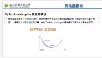
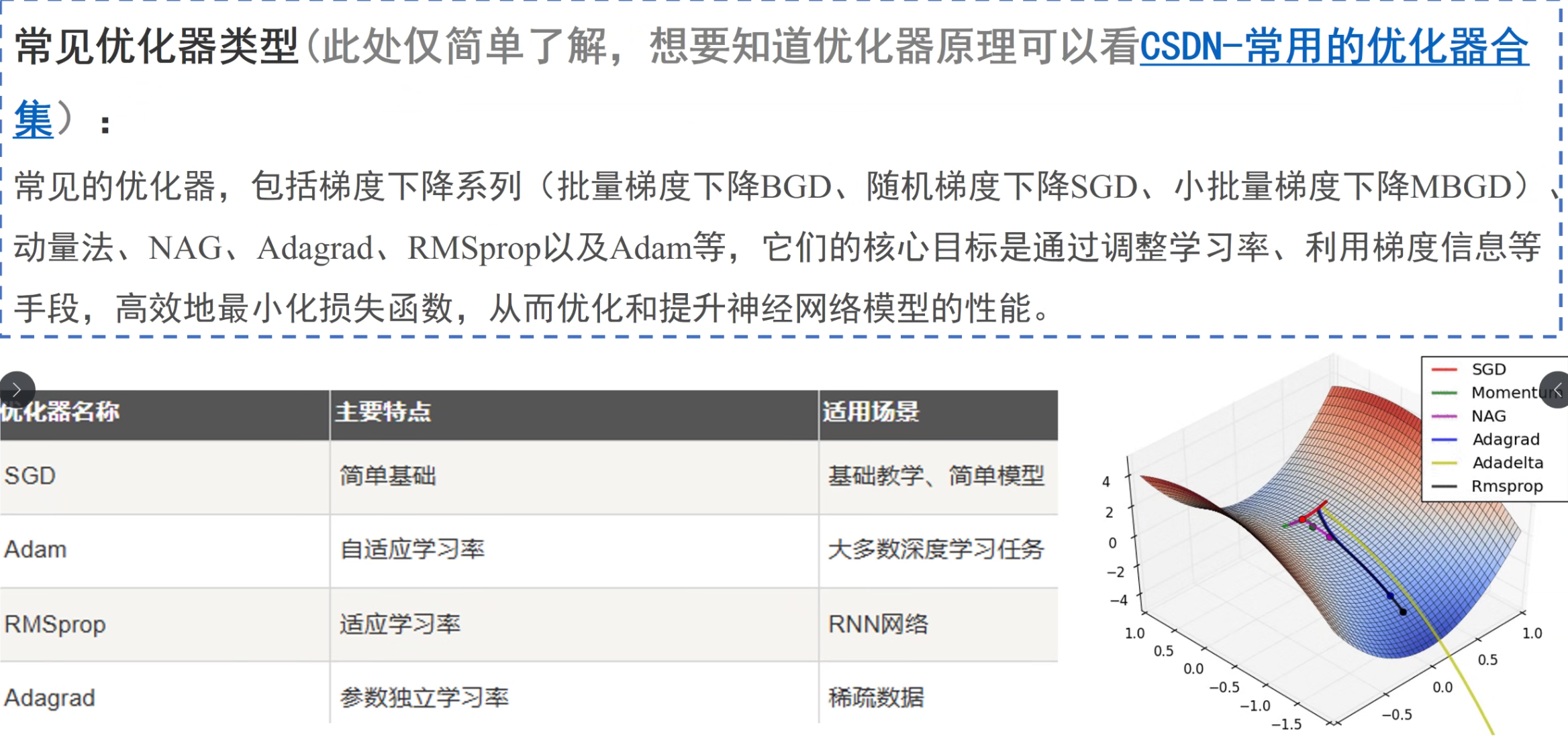
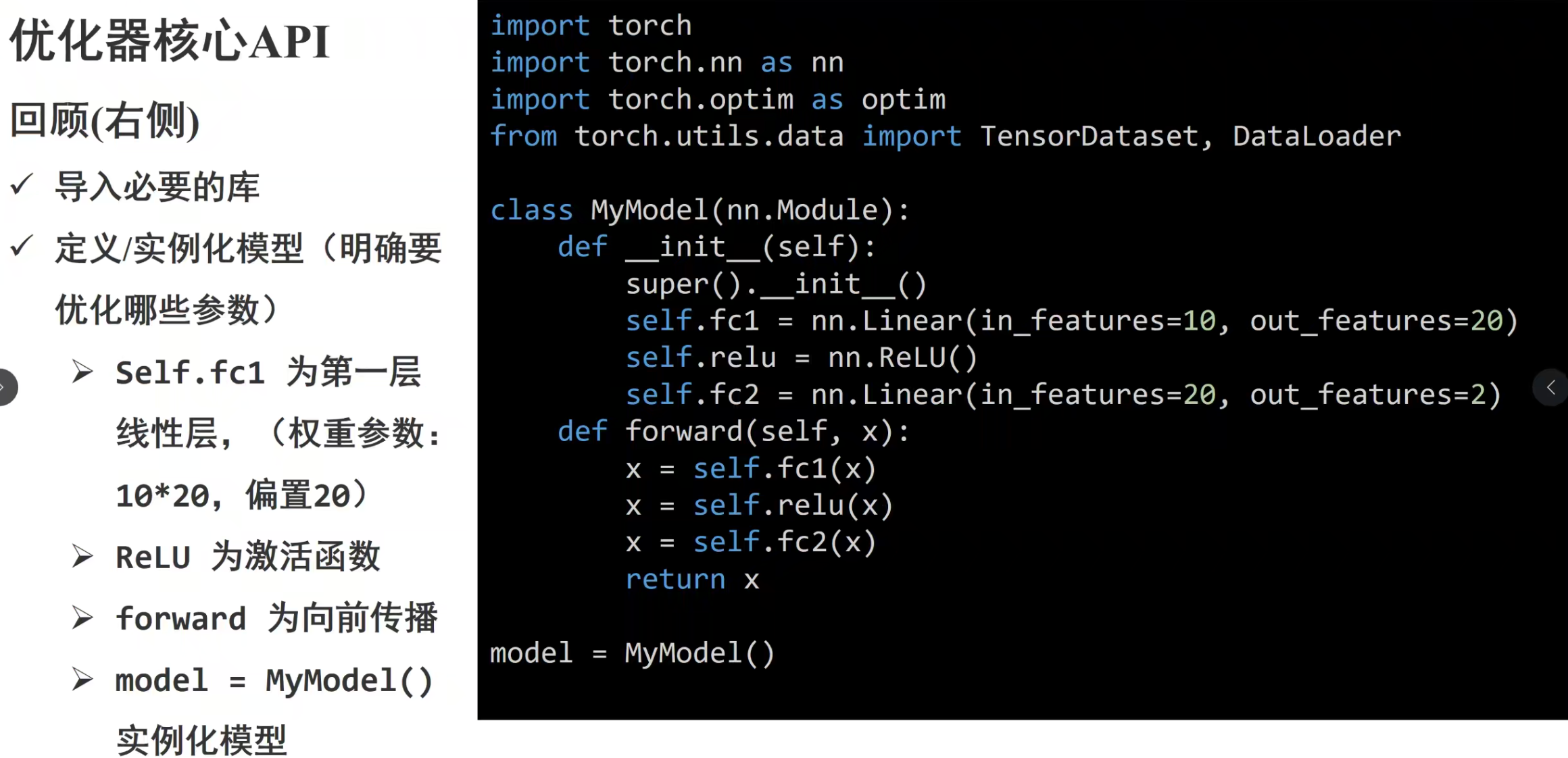
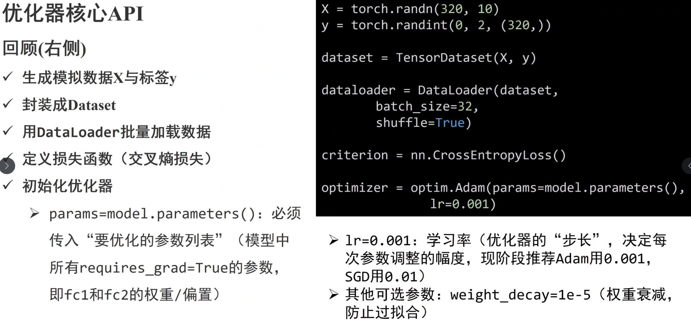
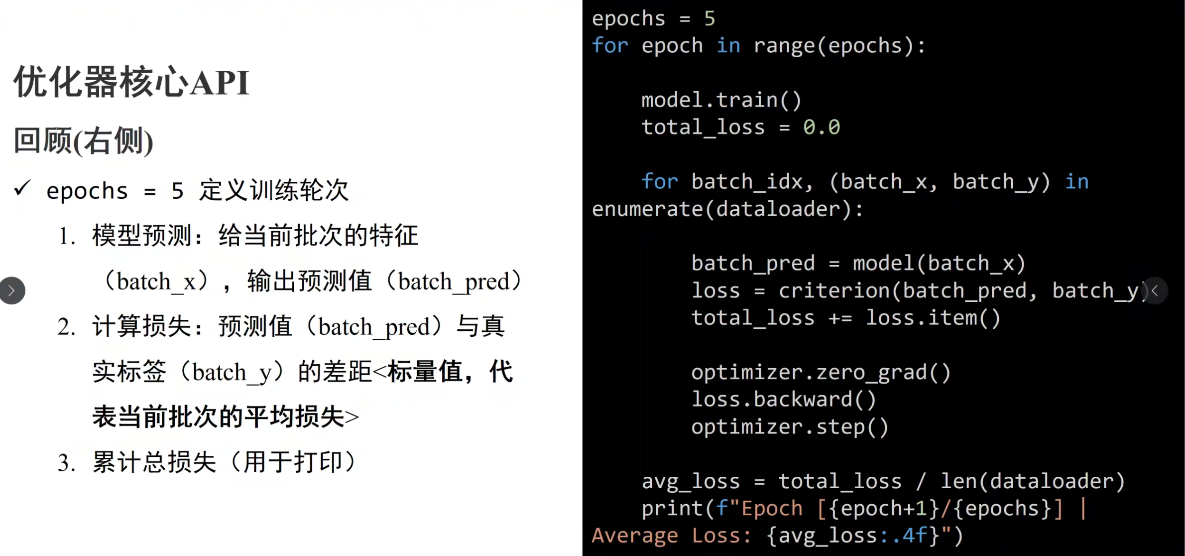
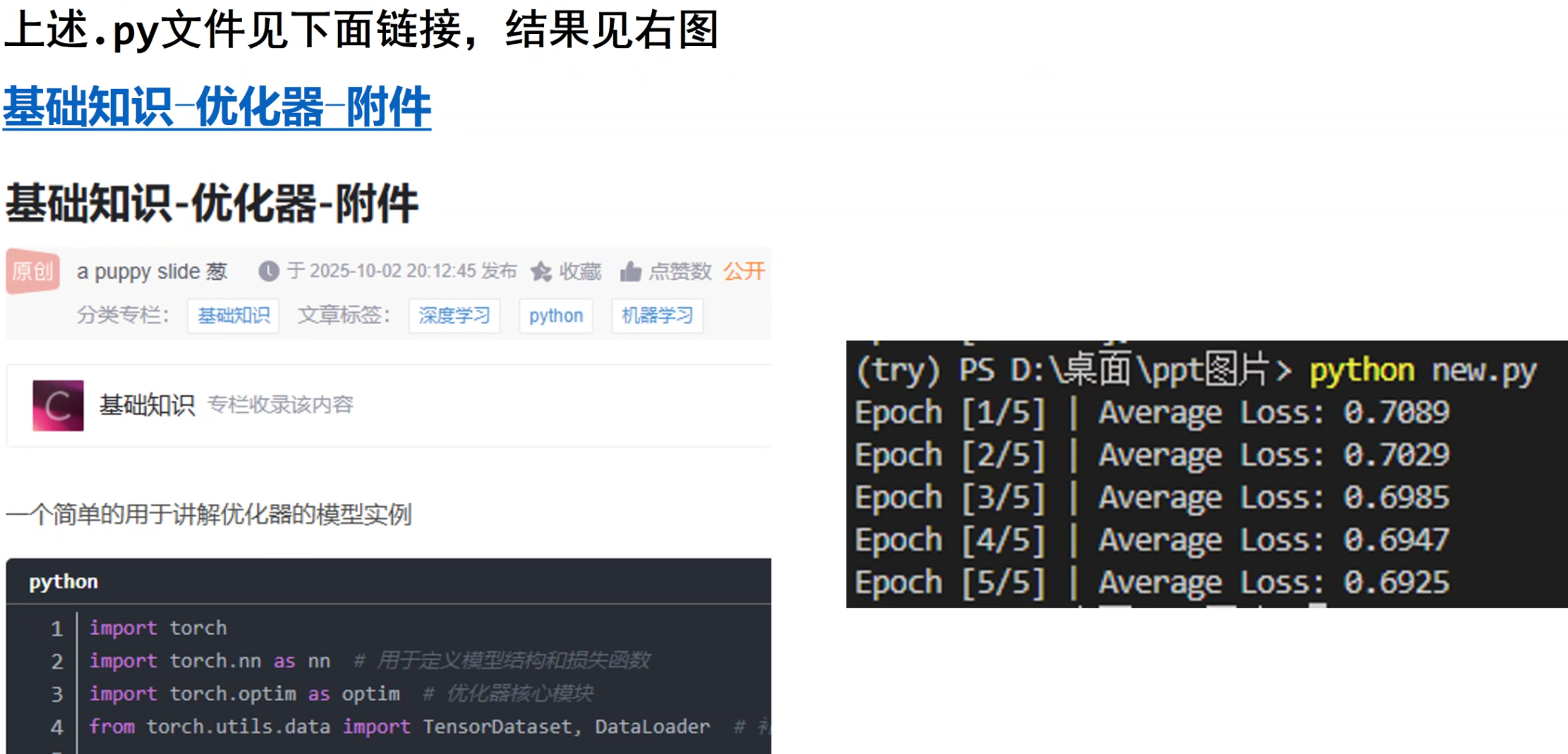
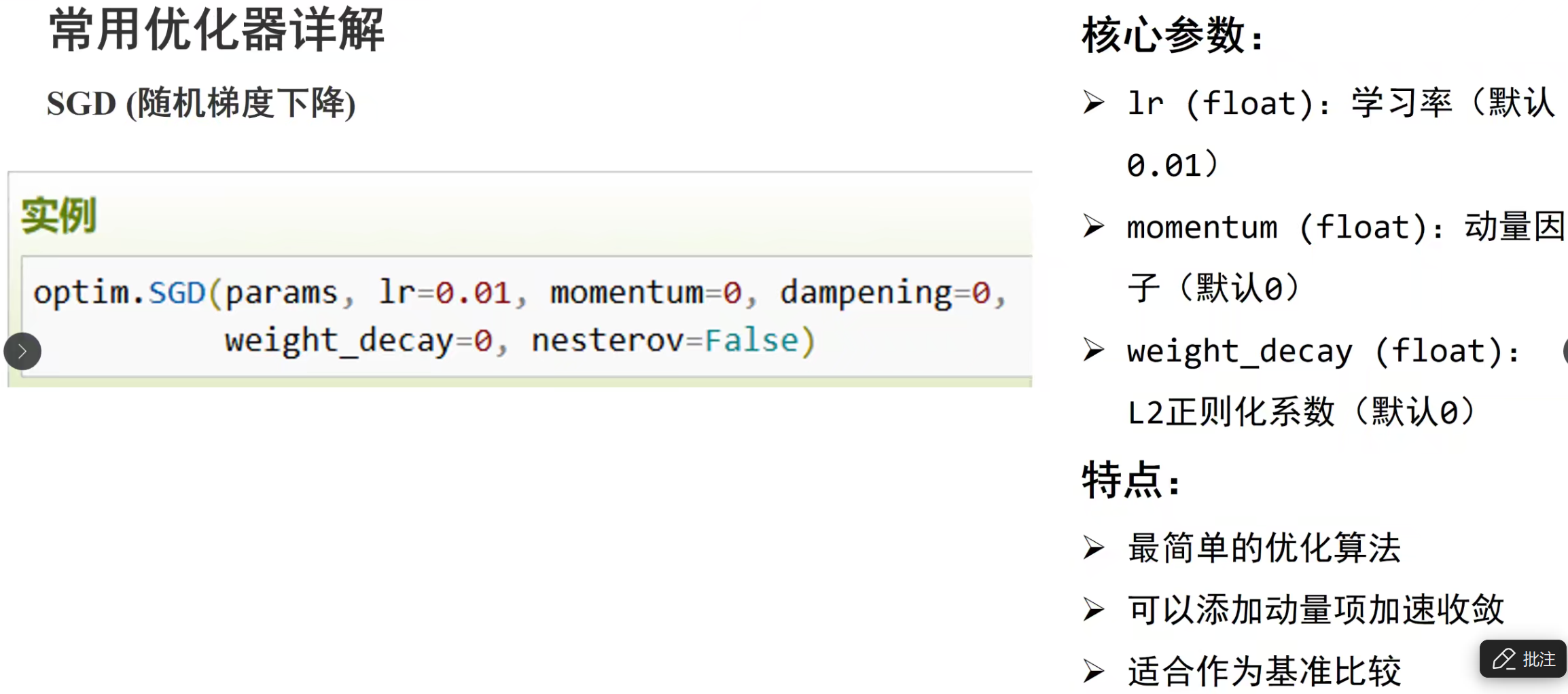
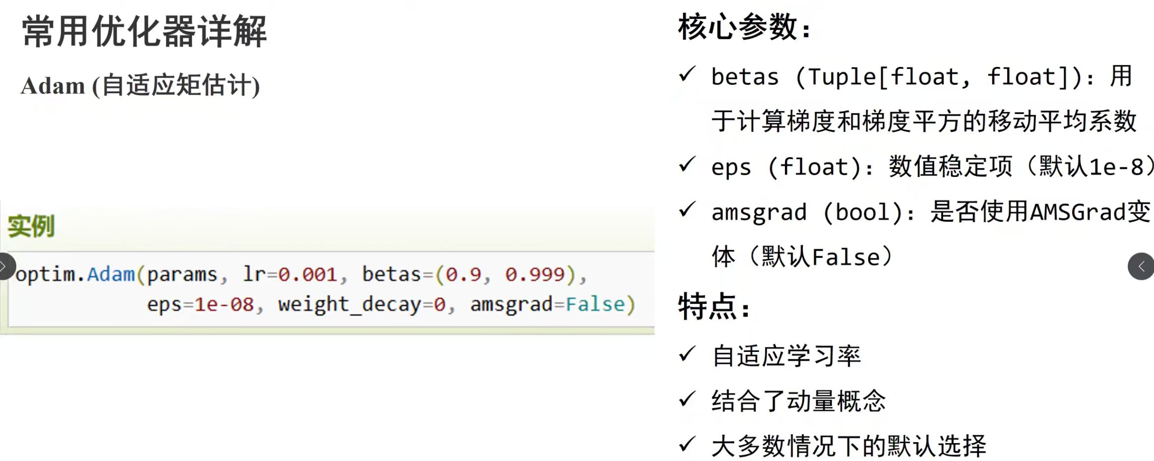
优化器模块
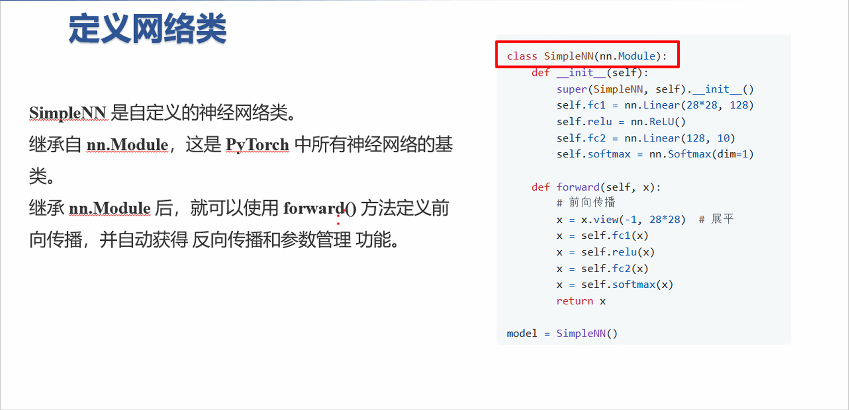
PyTorch 神经网络基础:__init__ 与 forward 方法详解 在 PyTorch 中,自定义神经网络类通常继承自 nn.Module,核心方法是 __init__ 和 forward。下面以一个简单的全连接网络为例进行讲解。
1. 模型代码示例 1 2 3 4 5 6 7 8 9 10 11 12 13 14 15 16 17 18 19 20 21 22 23 import torchimport torch.nn as nnclass SimpleNN (nn.Module): def __init__ (self ): super (SimpleNN, self ).__init__() self .fc1 = nn.Linear(28 *28 , 128 ) self .relu = nn.ReLU() self .fc2 = nn.Linear(128 , 10 ) self .softmax = nn.Softmax(dim=1 ) def forward (self, x ): x = x.view(-1 , 28 *28 ) x = self .fc1(x) x = self .relu(x) x = self .fc2(x) x = self .softmax(x) return x model = SimpleNN()
2. 方法详解 2.1 __init__ 方法 作用 :定义网络的各层,包括线性层、卷积层、激活函数等。
特点 :
仅声明网络结构,不进行前向计算。 注册子模块,便于 PyTorch 自动管理参数。 2.2 forward 方法 作用 :定义数据的前向传播流程。
特点 :
输入 x x x PyTorch 自动重载 __call__ 方法,调用模型实例时会触发 forward。 示例 :
1 output = model(input_tensor)
1 model.forward(input_tensor)
3. 数据流说明 输入图像张量 x x x ( batch size , 784 ) (\text{batch size}, 784) ( batch size , 784 ) 经过第一个全连接层 fc1,输出 ( batch size , 128 ) (\text{batch size}, 128) ( batch size , 128 ) 通过 ReLU 激活函数,增加非线性。 经过第二个全连接层 fc2,输出 ( batch size , 10 ) (\text{batch size}, 10) ( batch size , 10 ) 通过 Softmax 将输出转为概率分布,适合分类任务。 这种结构是典型的全连接神经网络(MLP)分类模型。
这种结构是典型的全连接神经网络(MLP)分类模型。
4. 补充说明 nn.Linear(in_features, out_features):创建全连接层,将输入特征维度 i n _ f e a t u r e s in\_features in _ f e a t u res o u t _ f e a t u r e s out\_features o u t _ f e a t u res nn.ReLU():激活函数,增加网络非线性能力。nn.Softmax(dim=1):对指定维度做归一化,使输出值可以看作概率分布。x.view(-1, 28*28):将输入张量展平成二维,-1 表示自动计算 batch size。在 PyTorch 中,所有 nn.Module 的子模块都会自动注册为模型参数,无需手动管理。 PyTorch 手写体图像识别教学 1. 导入必要库 1 2 3 4 5 6 7 8 9 import torchimport torch.nn as nnimport torch.optim as optimfrom torchvision import datasets, transformsfrom torch.utils.data import DataLoader
#@ 2. 数据预处理与加载
1 2 3 4 5 6 7 8 9 10 transform = transforms.Compose([ transforms.ToTensor(), transforms.Normalize((0.5 ,), (0.5 ,)) ]) train_dataset = datasets.MNIST(root='./data' , train=True , download=True , transform=transform) test_dataset = datasets.MNIST(root='./data' , train=False , download=True , transform=transform) train_loader = DataLoader(train_dataset, batch_size=64 , shuffle=True ) test_loader = DataLoader(test_dataset, batch_size=64 , shuffle=False )
3. 定义前馈神经网络 网络结构:
1 2 3 4 5 6 7 8 9 10 11 12 13 14 15 16 17 18 class SimpleNN (nn.Module): def __init__ (self ): super (SimpleNN, self ).__init__() self .fc1 = nn.Linear(28 *28 , 128 ) self .relu = nn.ReLU() self .fc2 = nn.Linear(128 , 10 ) self .softmax = nn.Softmax(dim=1 ) def forward (self, x ): x = x.view(-1 , 28 *28 ) x = self .fc1(x) x = self .relu(x) x = self .fc2(x) x = self .softmax(x) return x model = SimpleNN()
4. 定义损失函数和优化器 多分类交叉熵损失
1 2 criterion = nn.CrossEntropyLoss() optimizer = optim.SGD(model.parameters(), lr=0.01 )
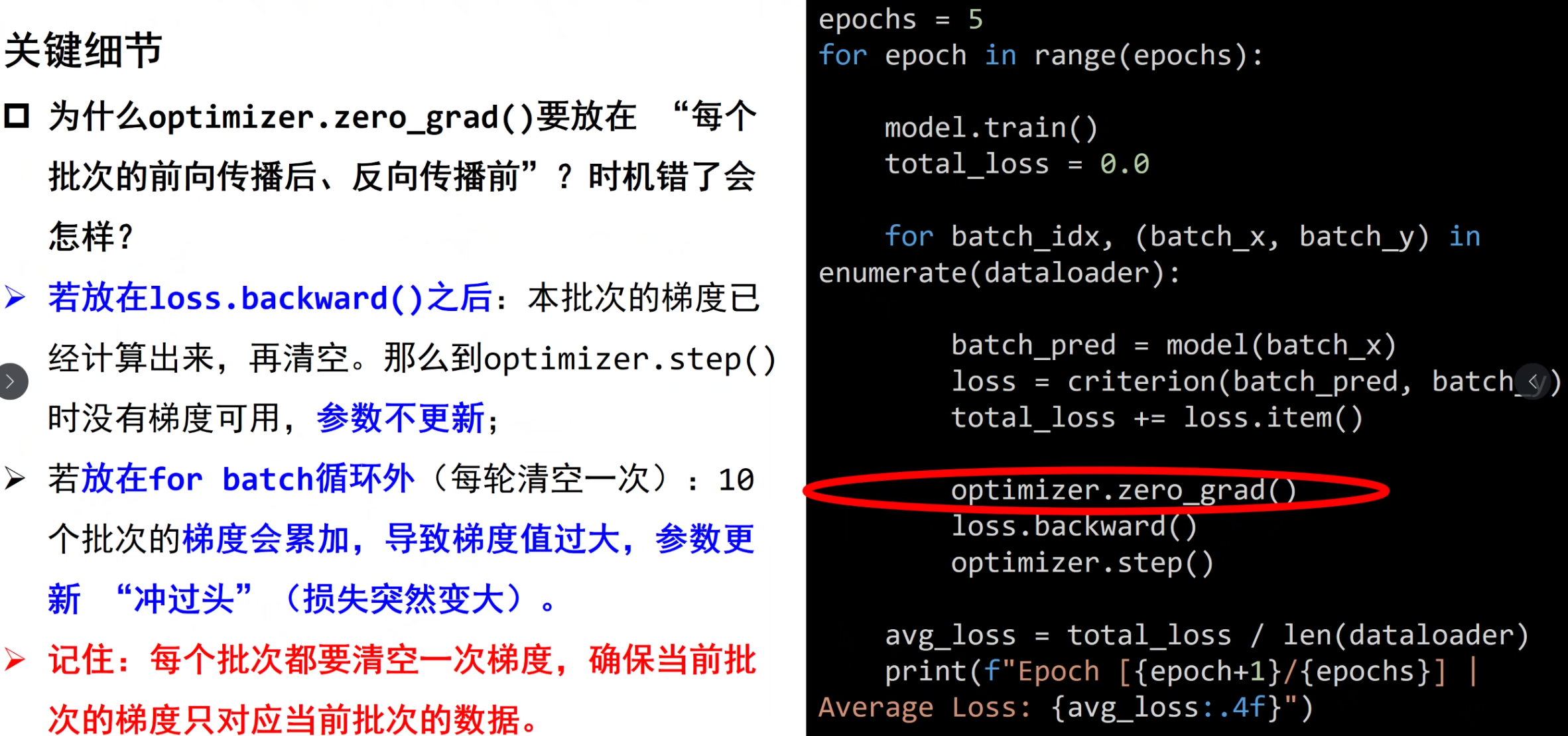
5. 模型训练 训练流程: 1. 前向传播: 计算预测输出 2. 计算损失 3. 反向传播 4. 参数更新 1 2 3 4 5 6 7 8 9 10 11 12 13 num_epochs = 5 for epoch in range (num_epochs): running_loss = 0.0 for images, labels in train_loader: outputs = model(images) loss = criterion(outputs, labels) optimizer.zero_grad() loss.backward() optimizer.step() running_loss += loss.item() print (f"Epoch [{epoch+1 } /{num_epochs} ], Loss: {running_loss/len (train_loader):.4 f} " )
6. 测试模型准确率 在测试集上评估模型性能
1 2 3 4 5 6 7 8 9 10 correct = 0 total = 0 with torch.no_grad(): for images, labels in test_loader: outputs = model(images) _, predicted = torch.max (outputs.data, 1 ) total += labels.size(0 ) correct += (predicted == labels).sum ().item() print (f'Test Accuracy: {100 * correct / total:.2 f} %' )
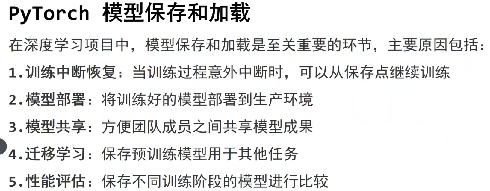
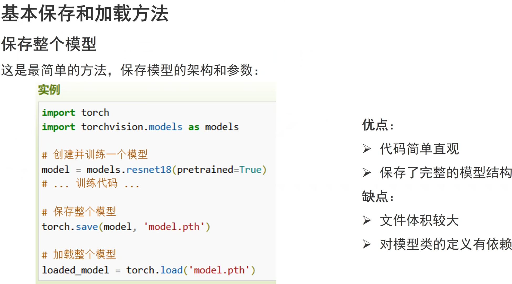
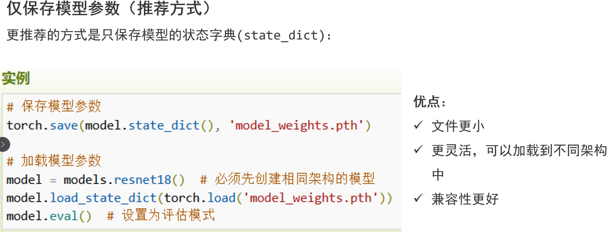
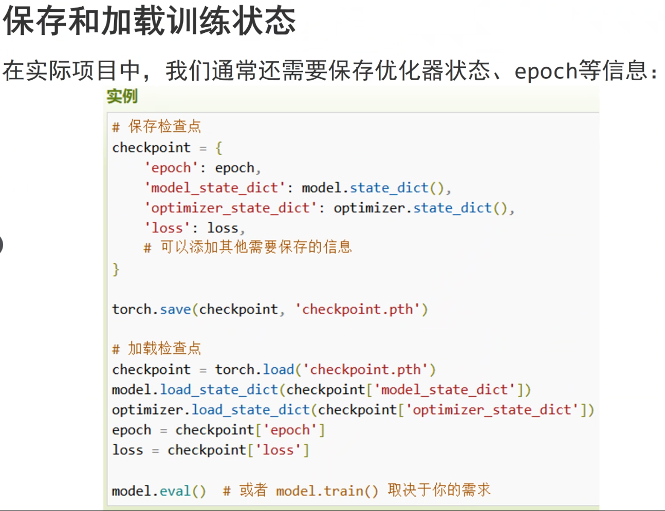
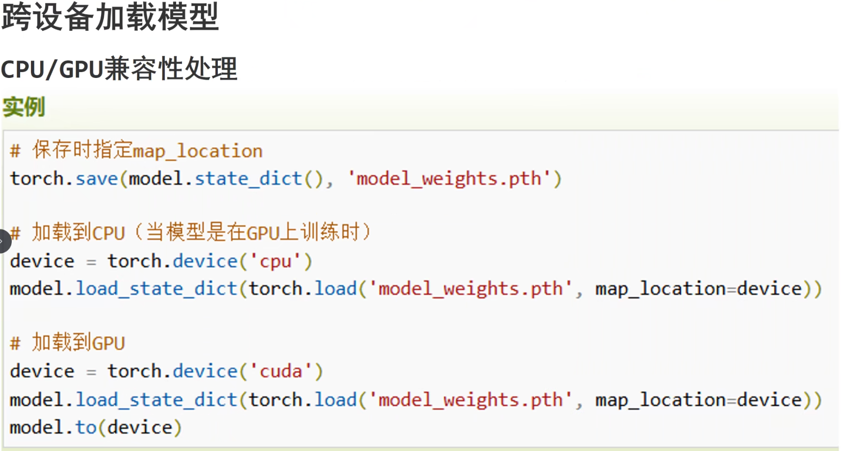
模型保存和加载
优点:保存了模型的完整结构
缺点:模型文件体积大
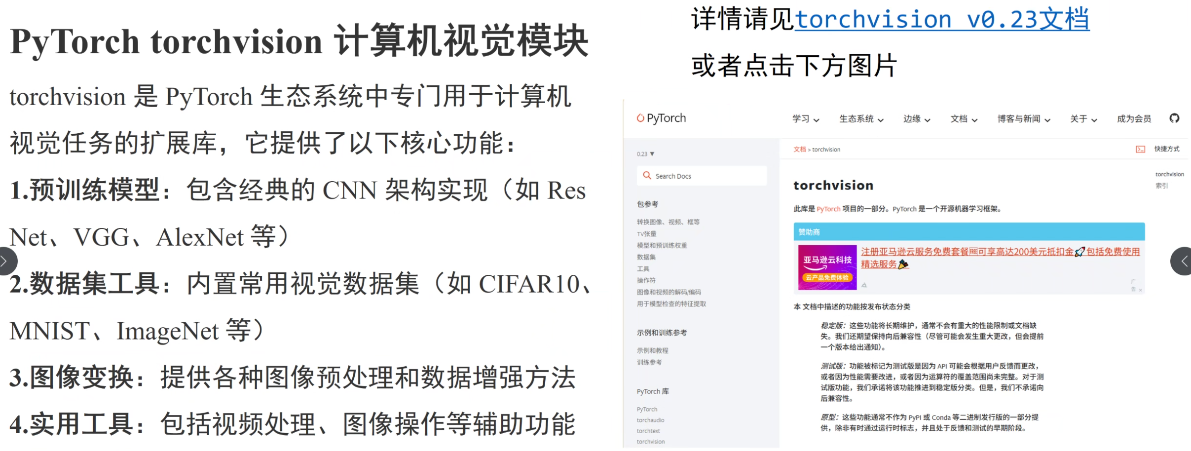
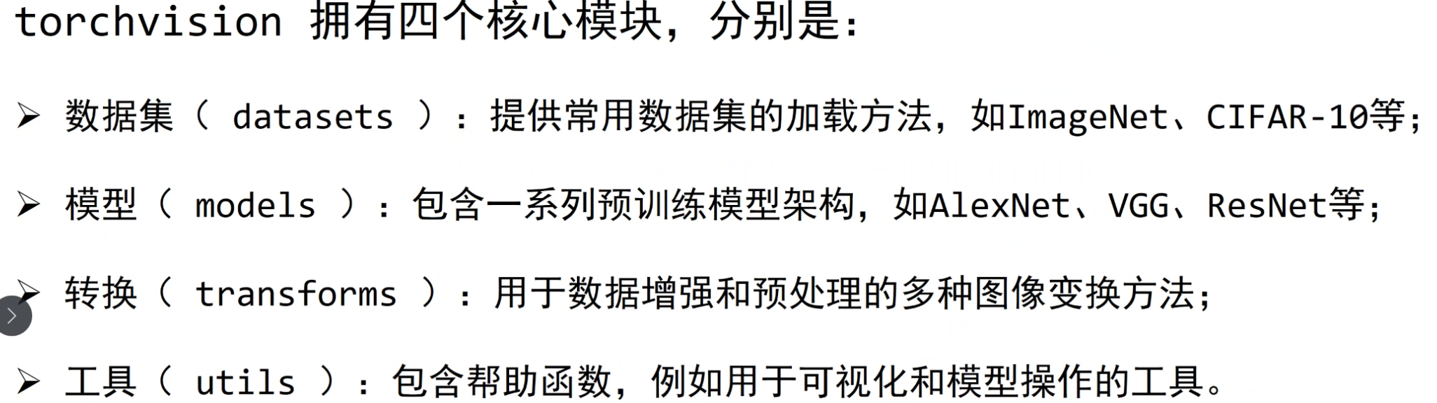
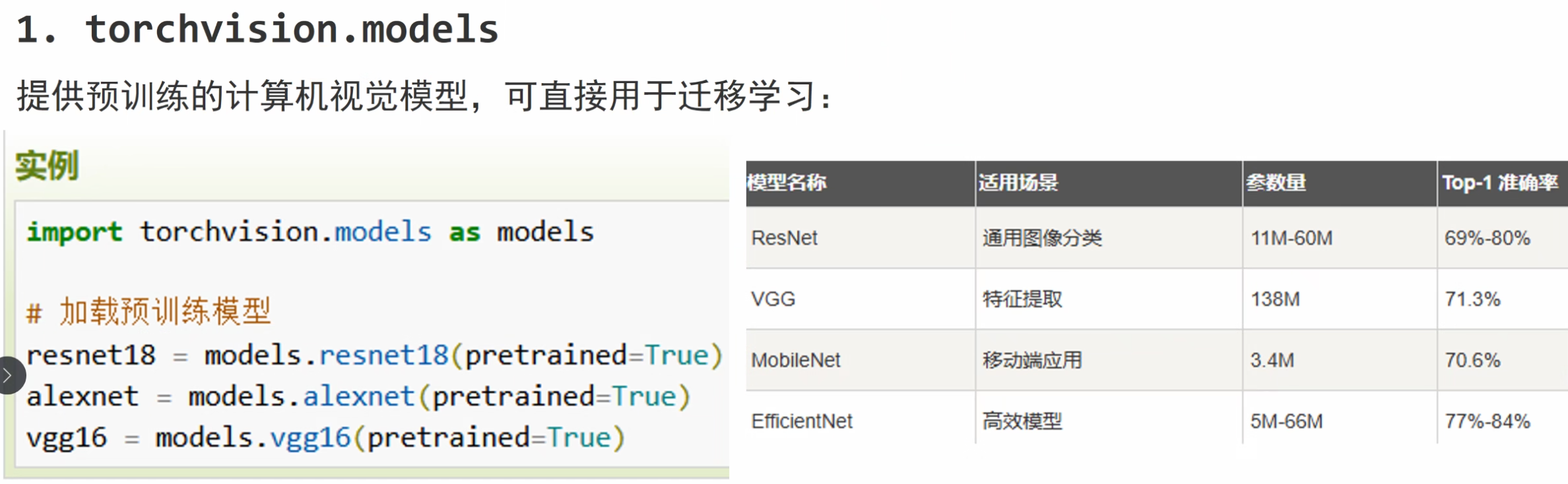
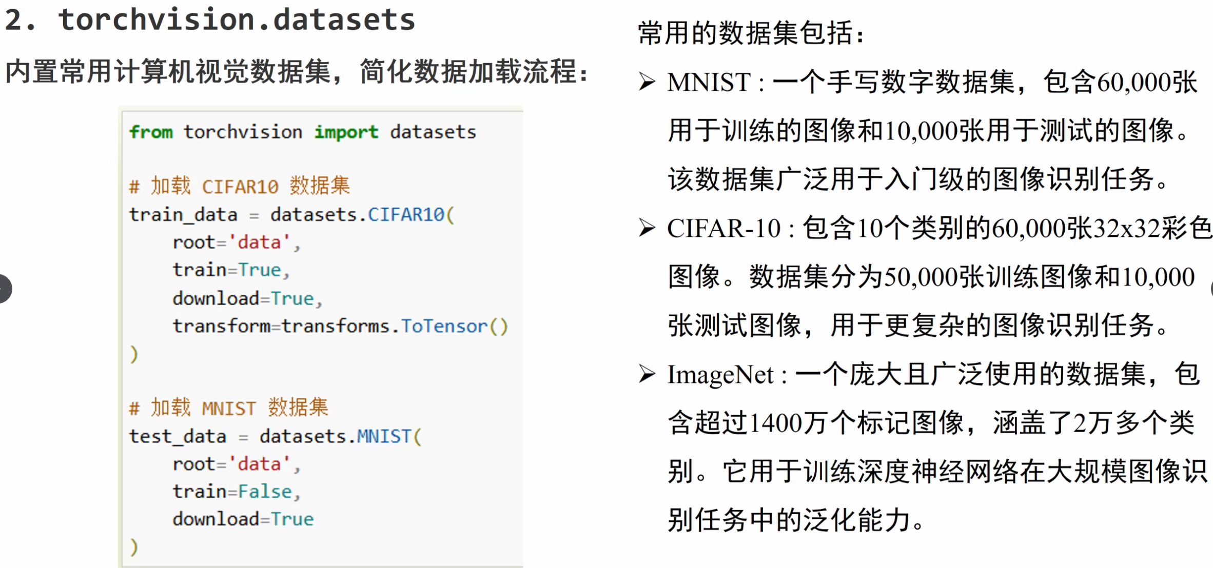
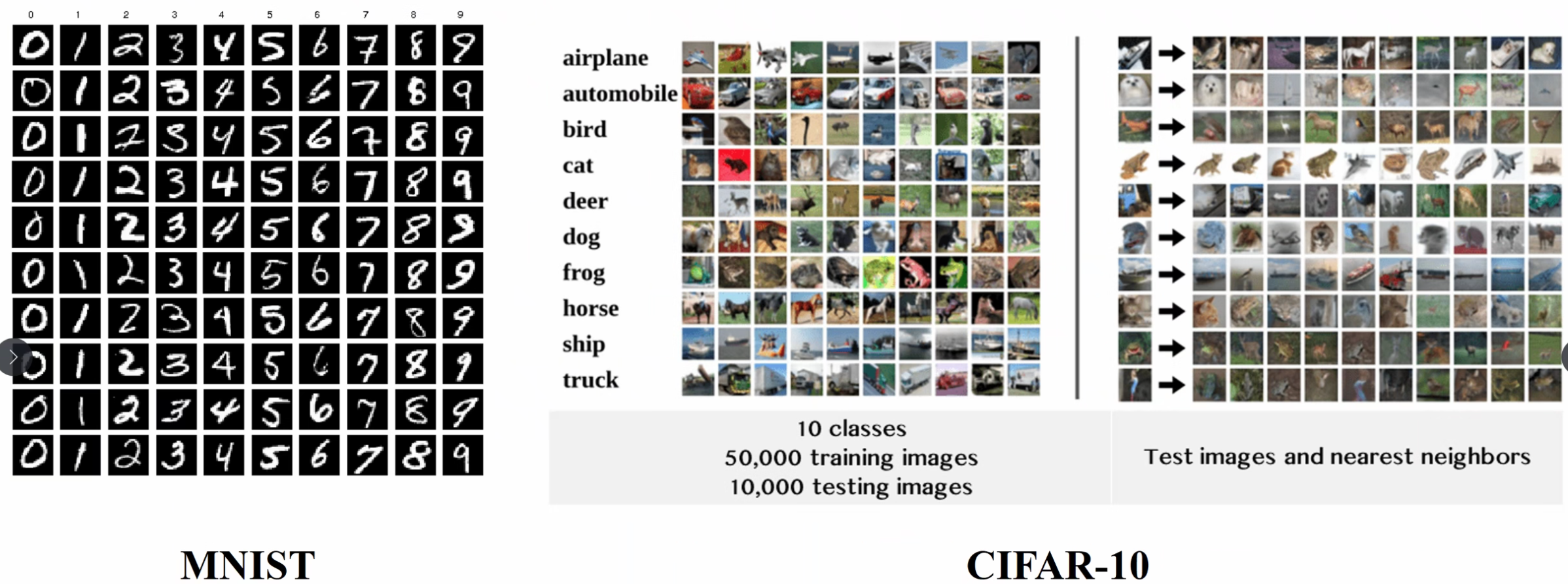
计算机视觉模块
torchvision — Torchvision 0.23 文档 - PyTorch 文档
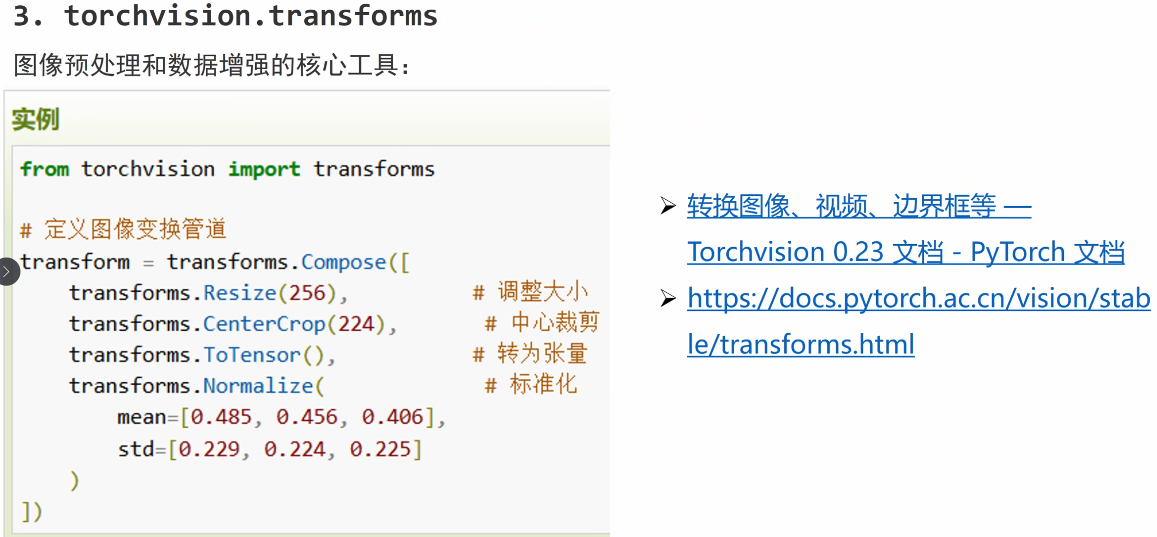
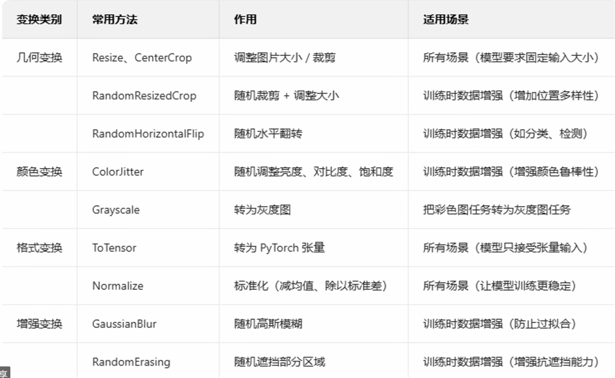
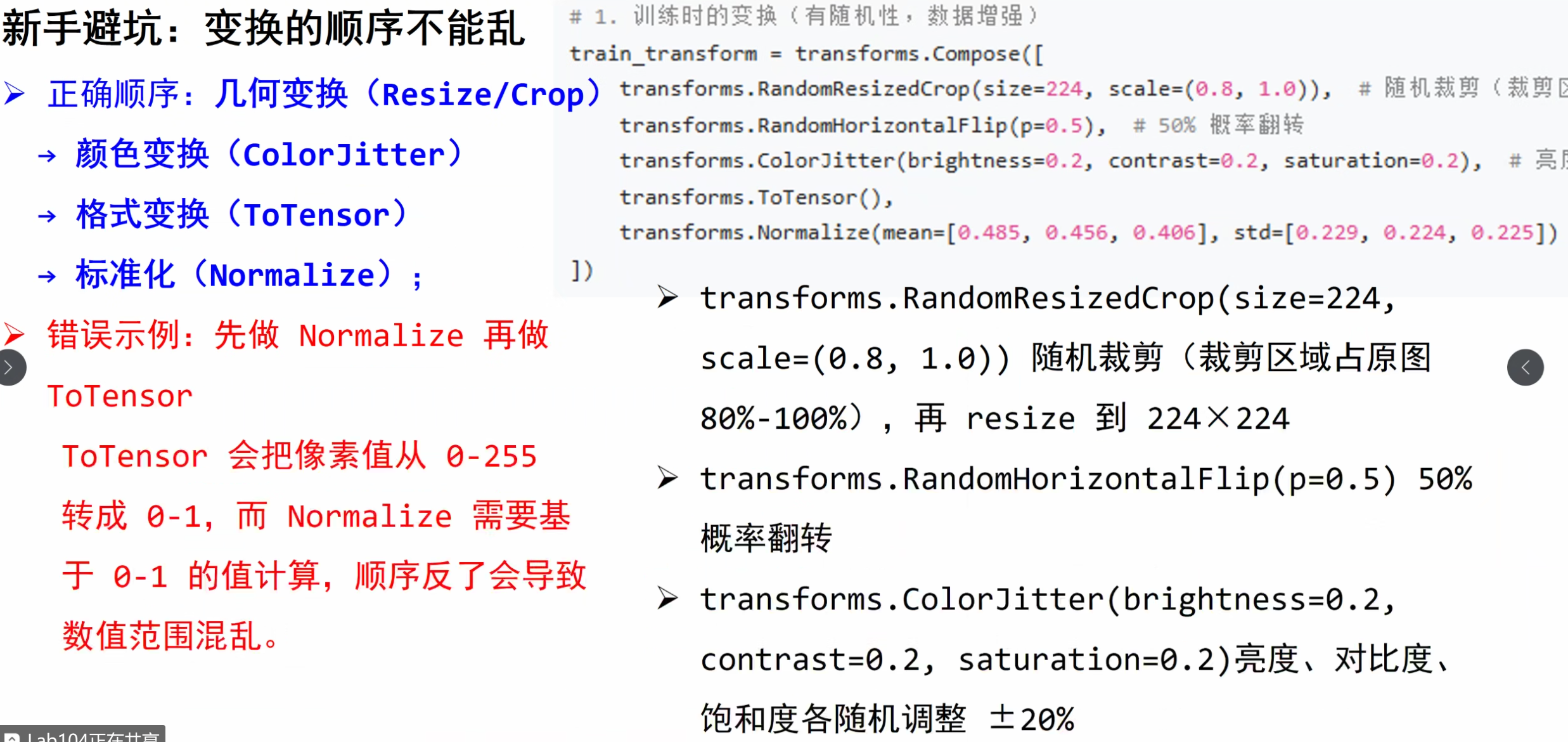
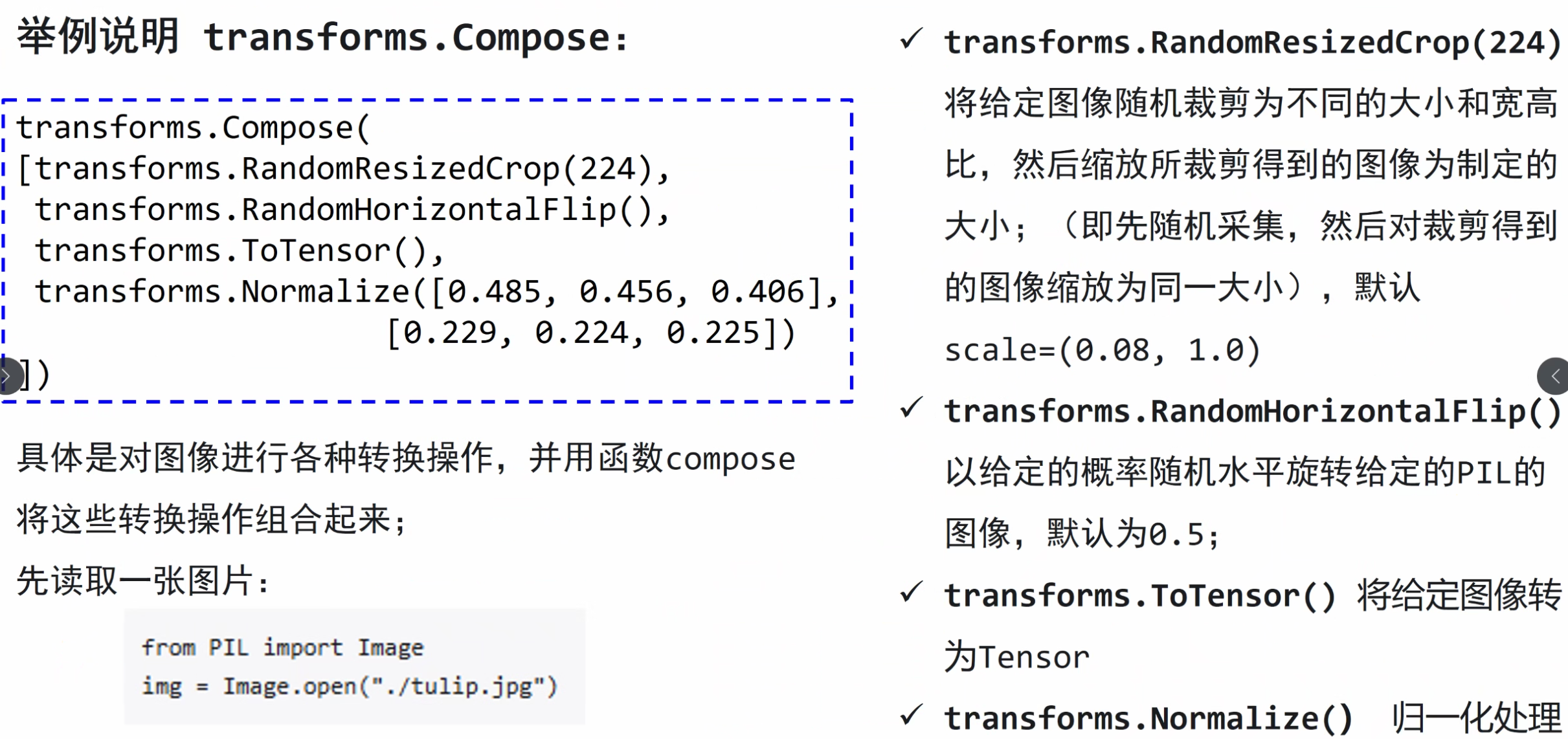
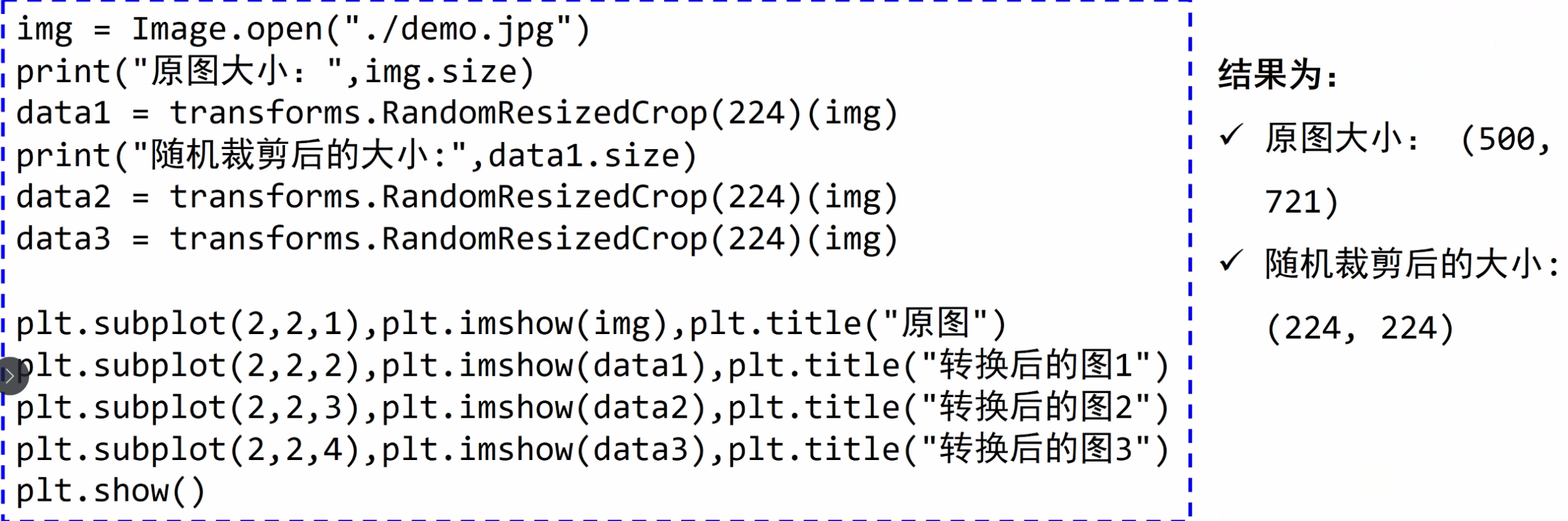
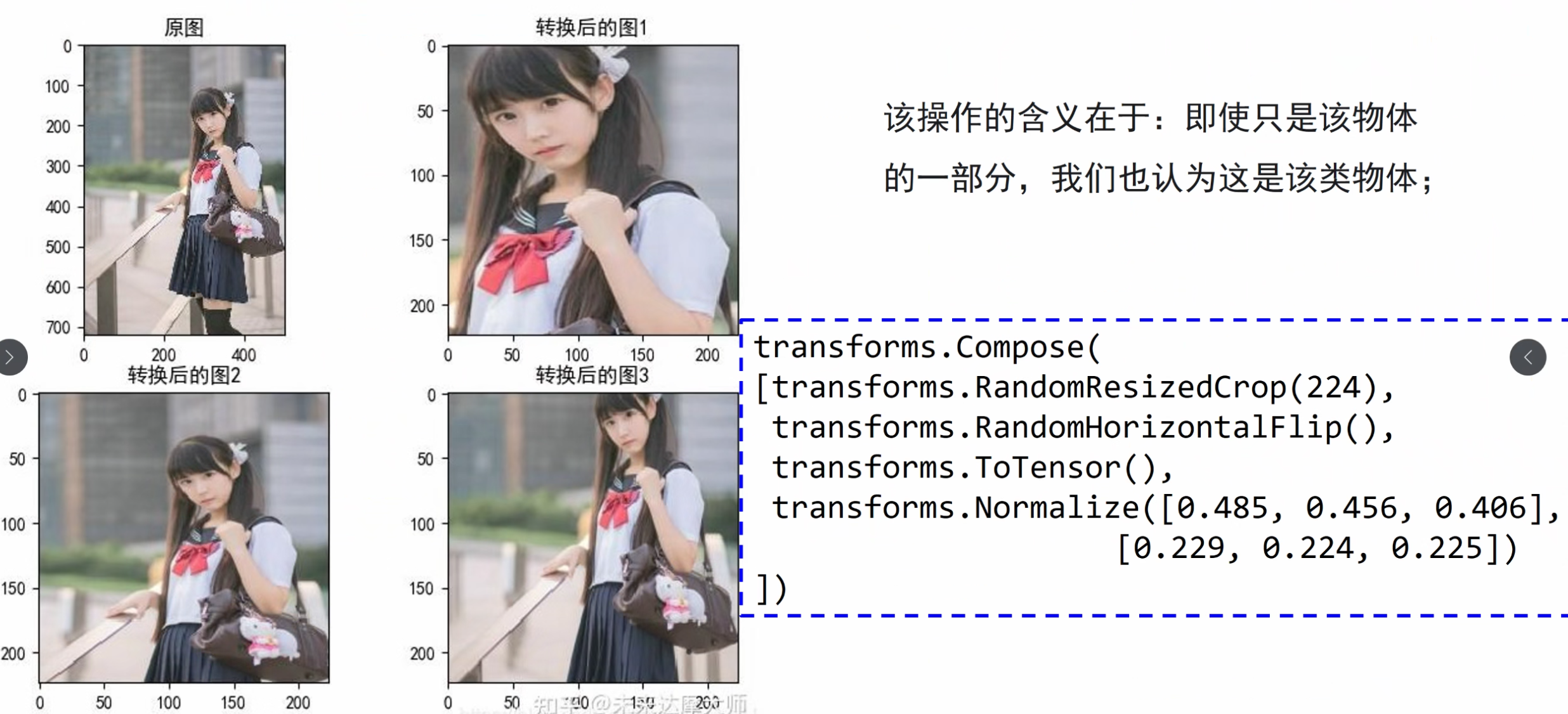
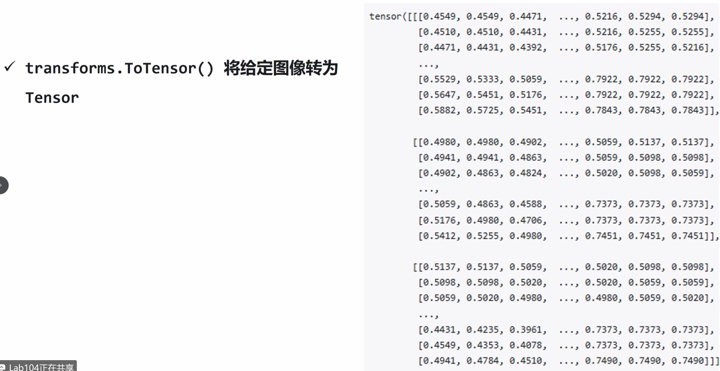
转换图像、视频、边界框等 — Torchvision 0.23 文档 - PyTorch 文档
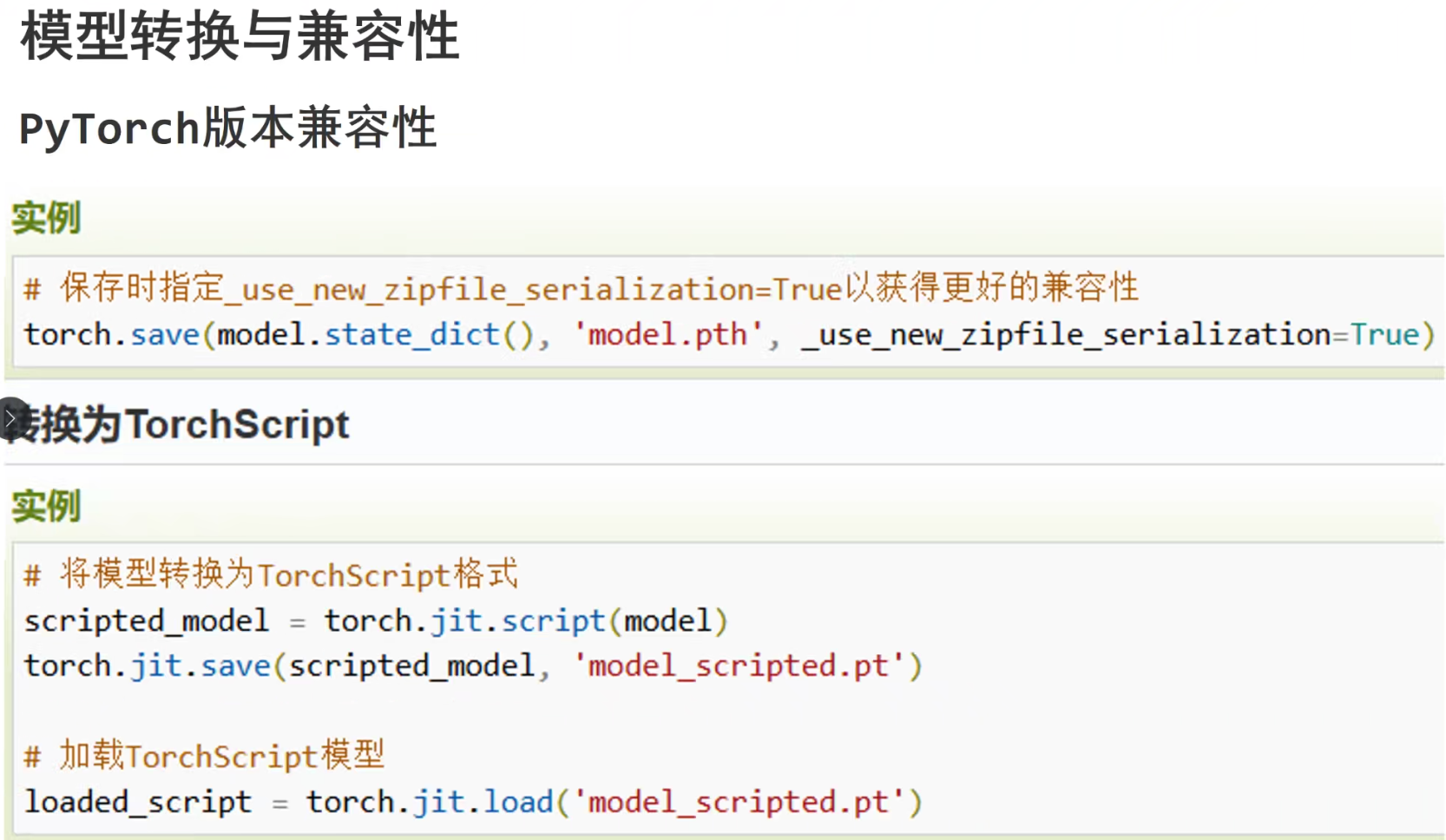
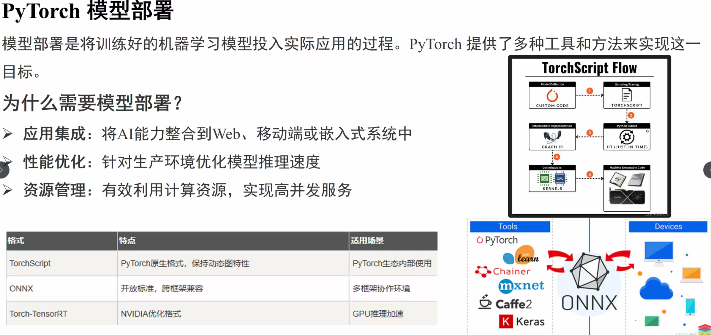
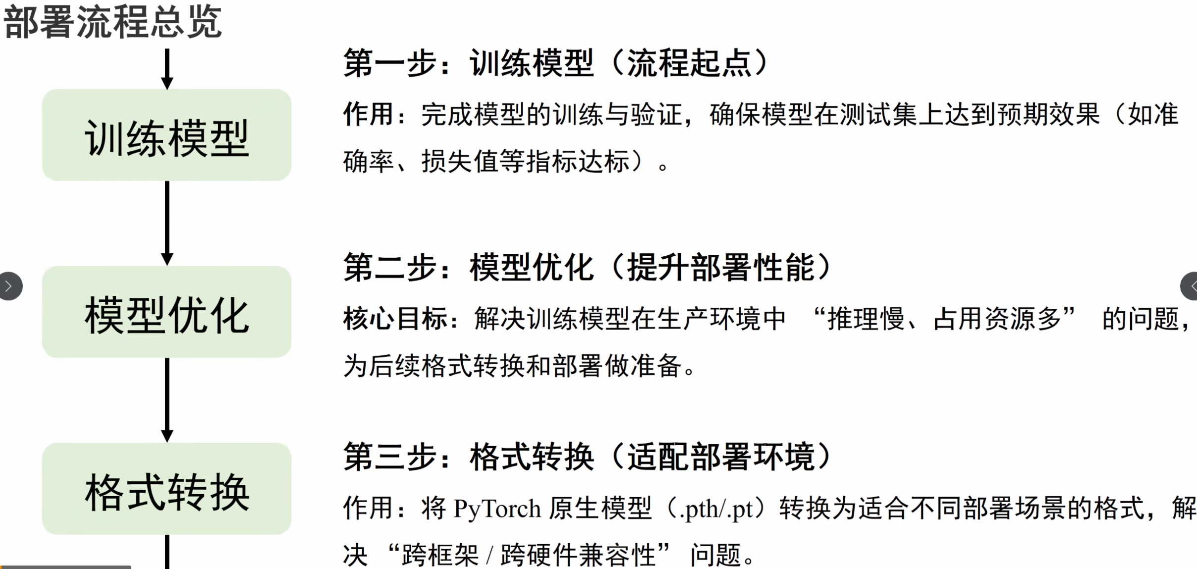
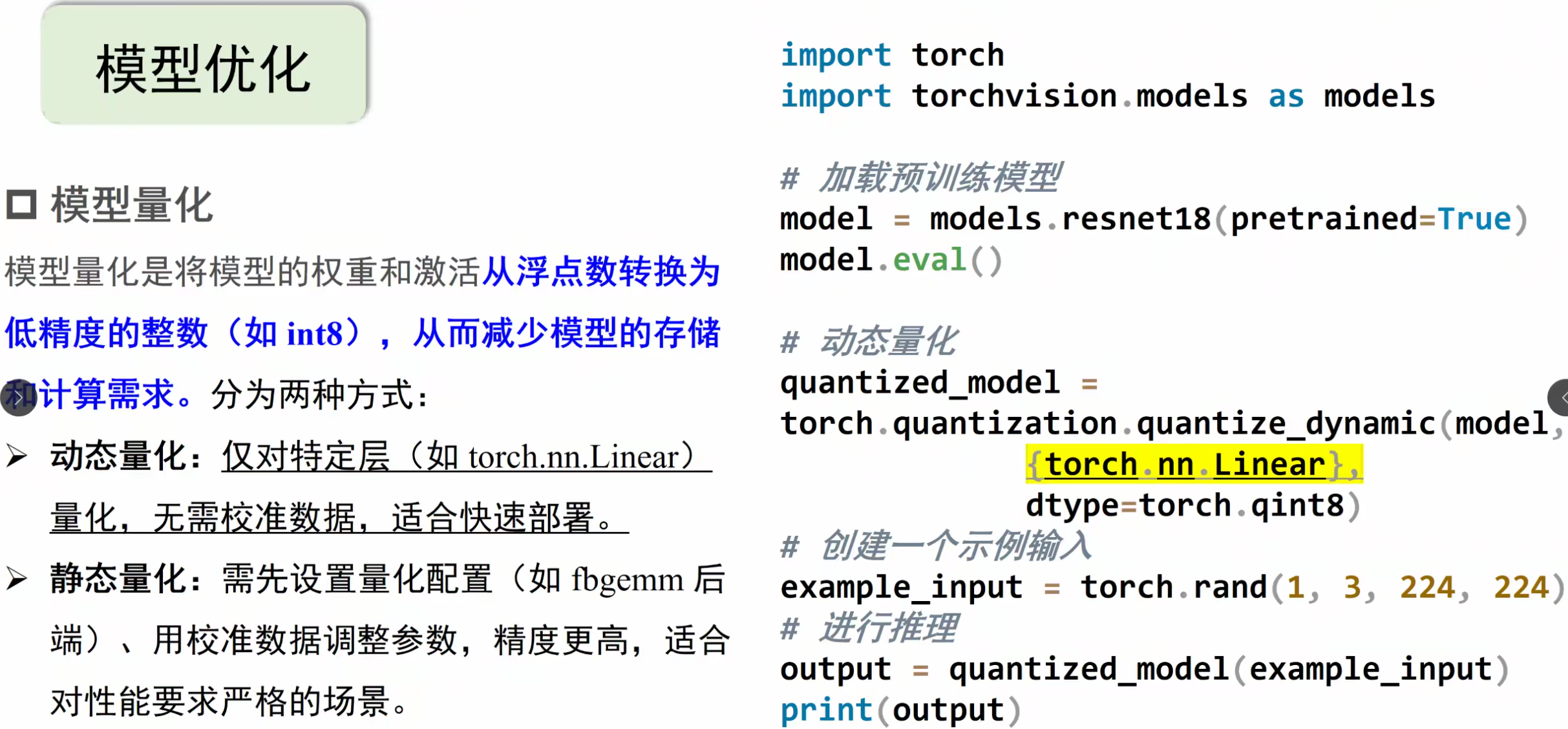
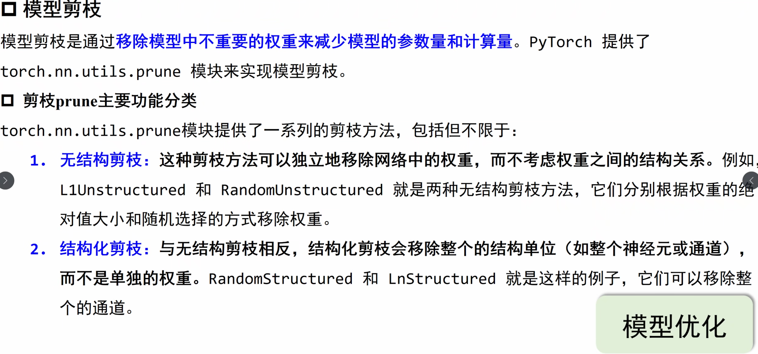
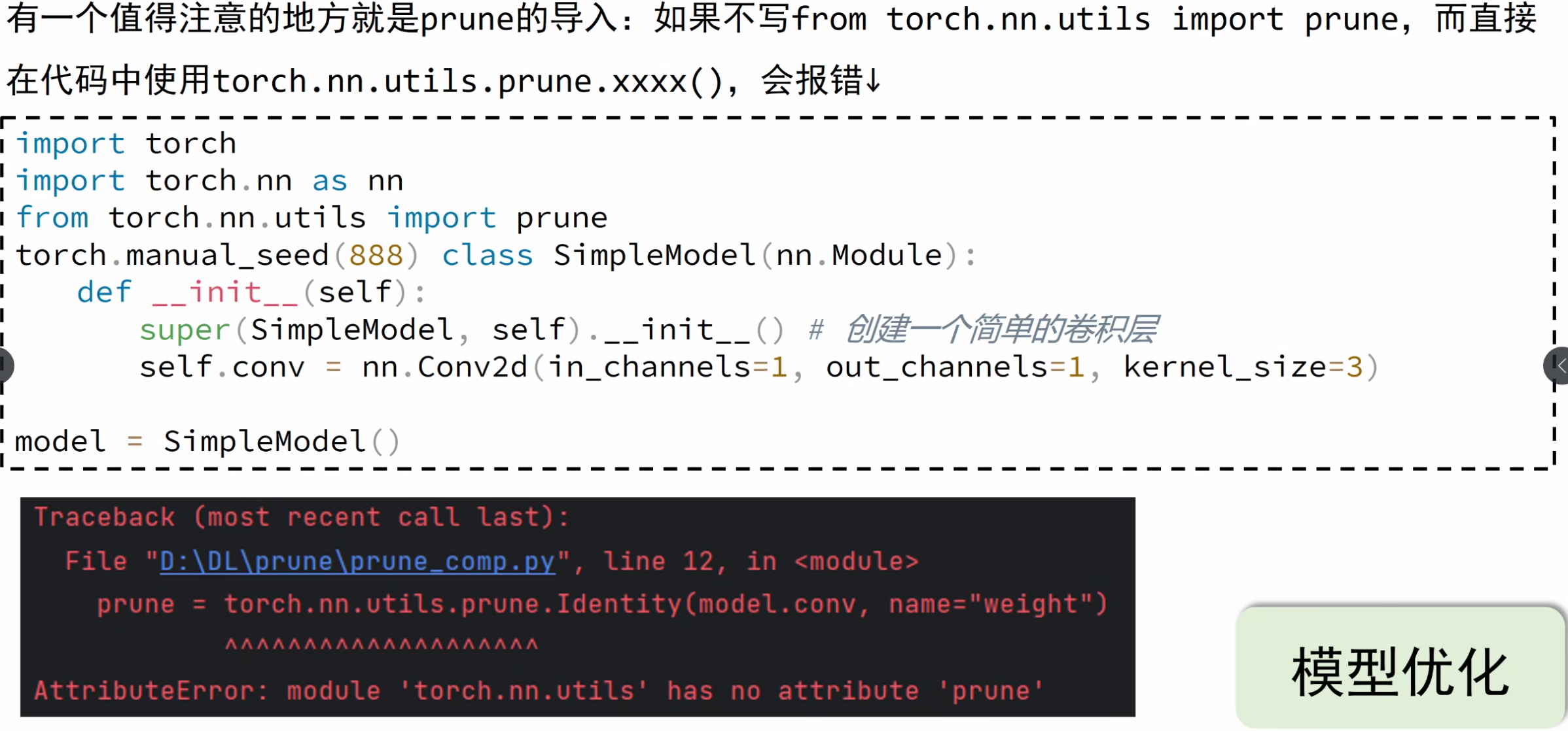
模型部署
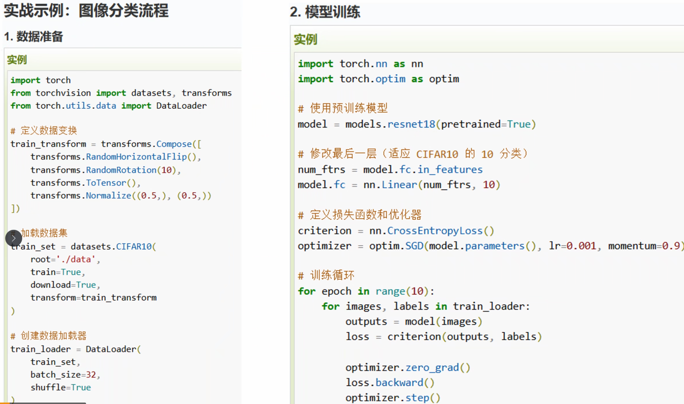
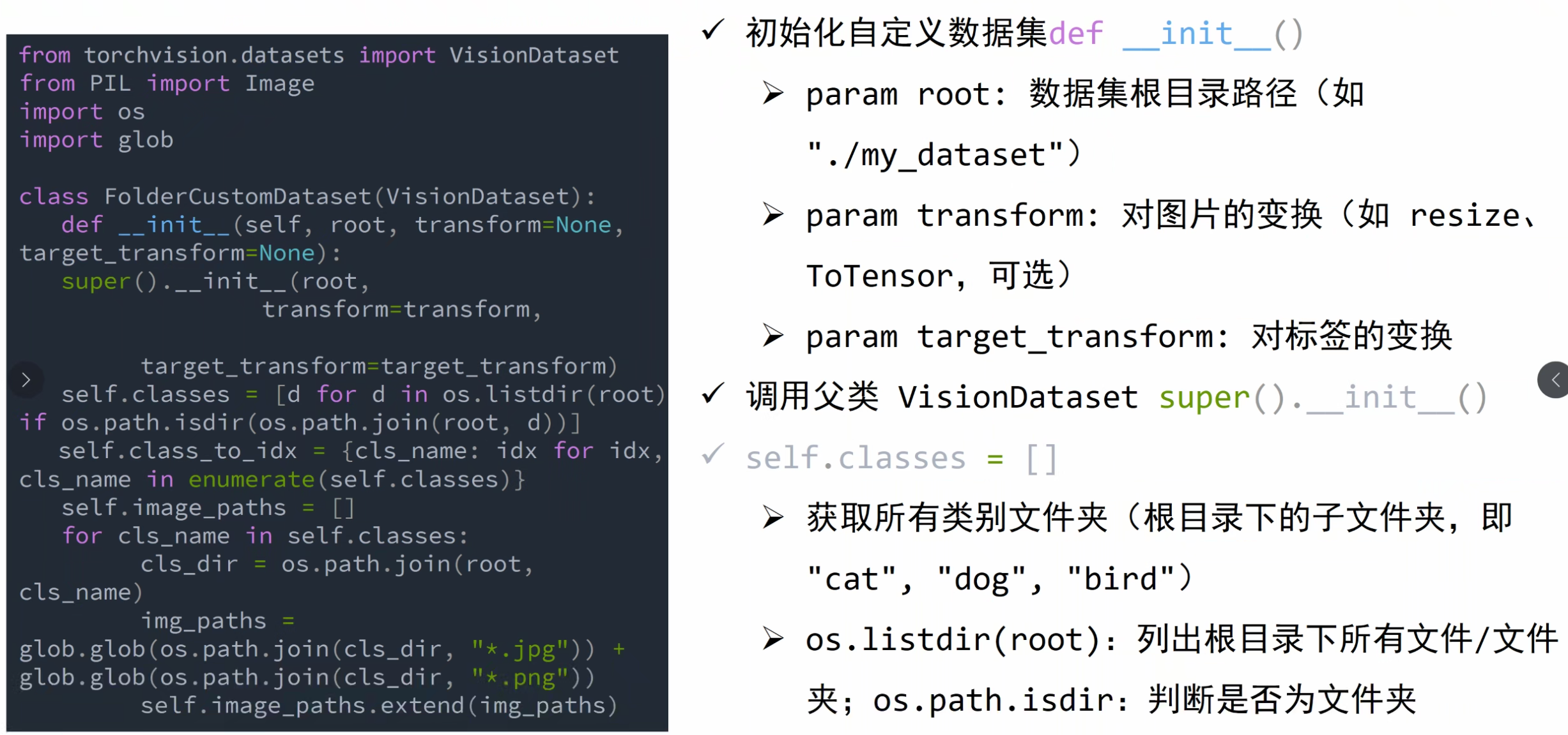
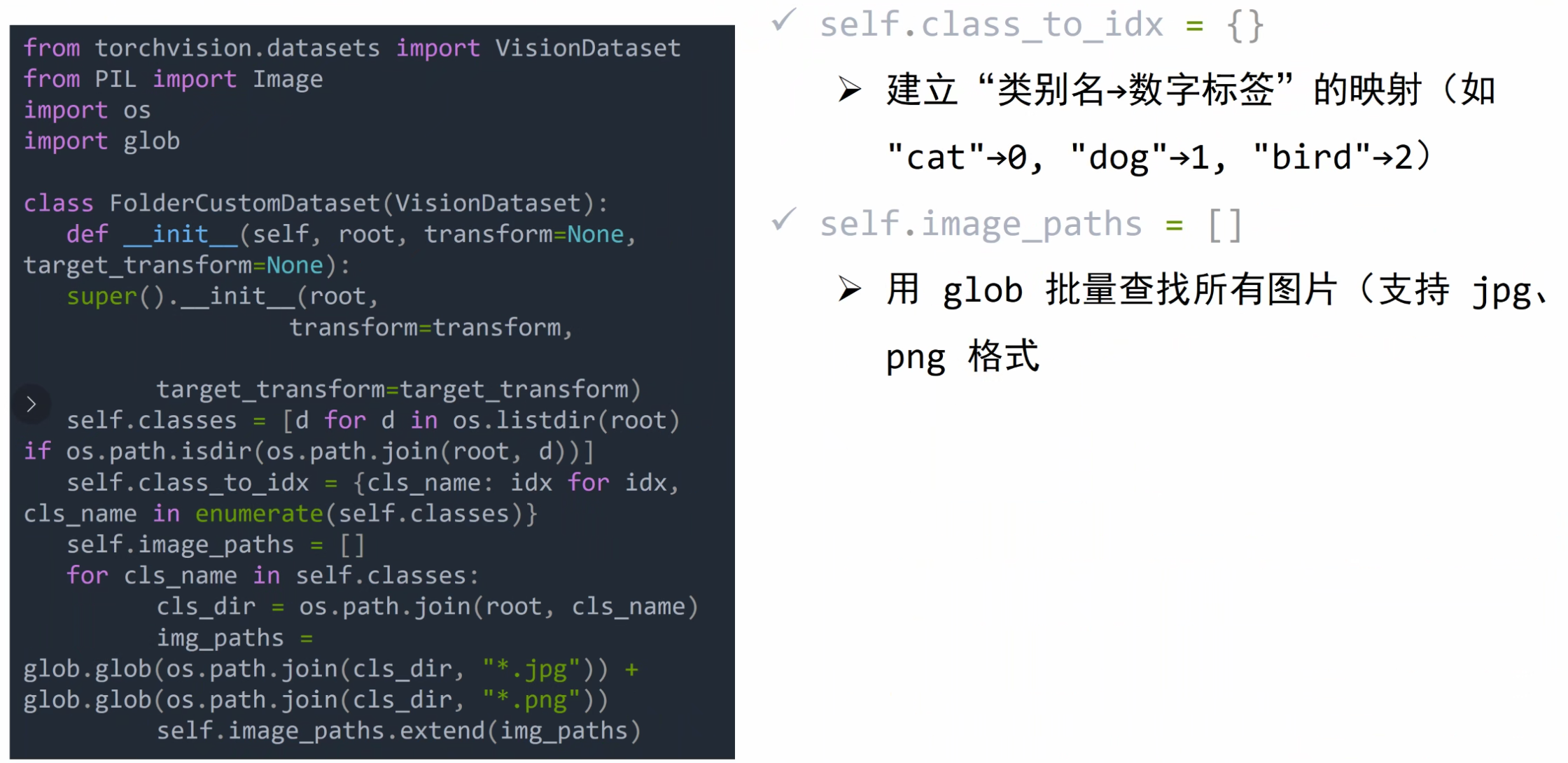
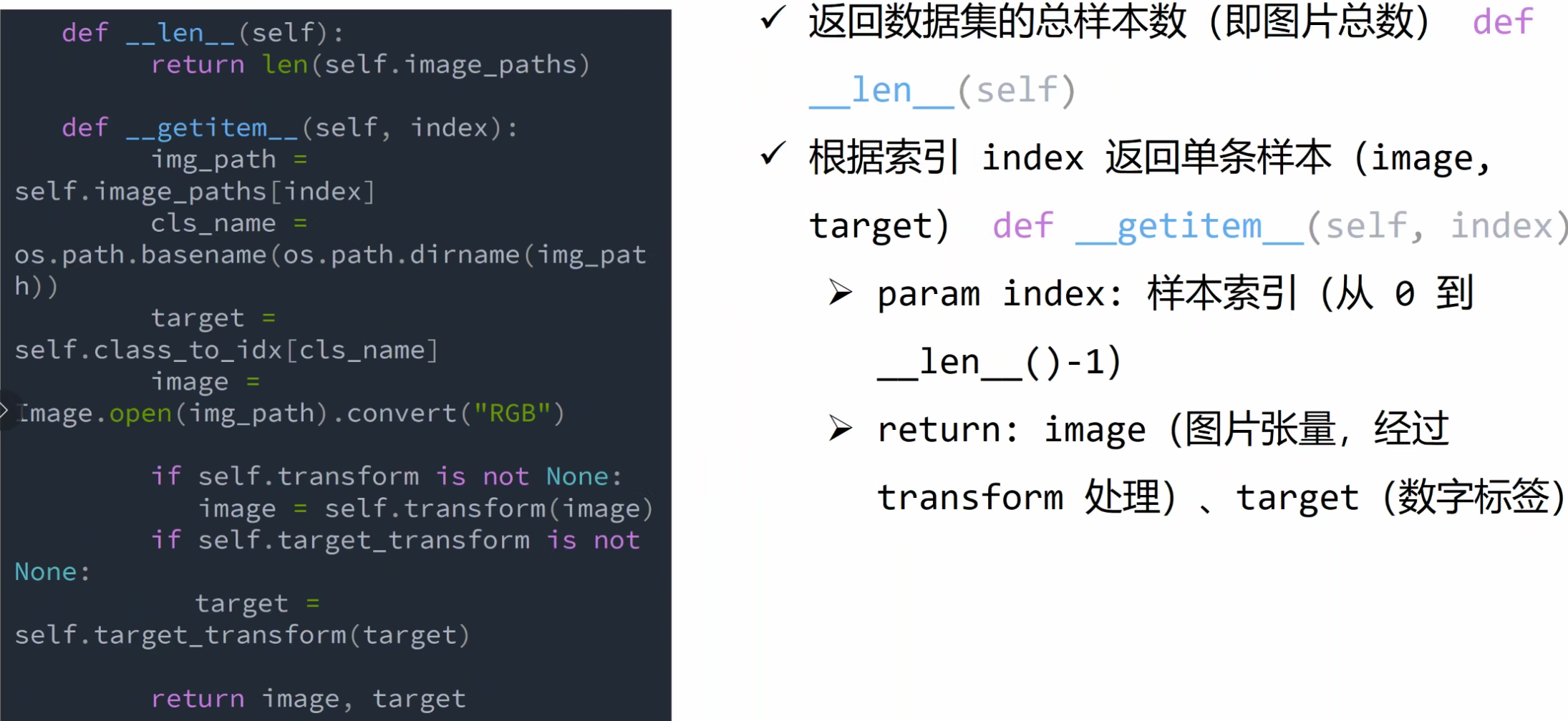
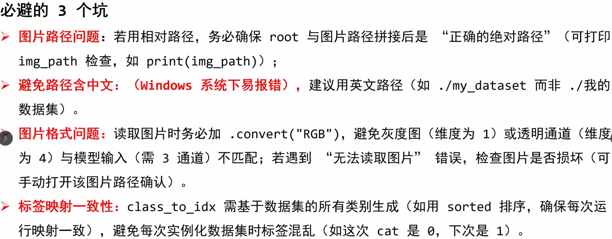
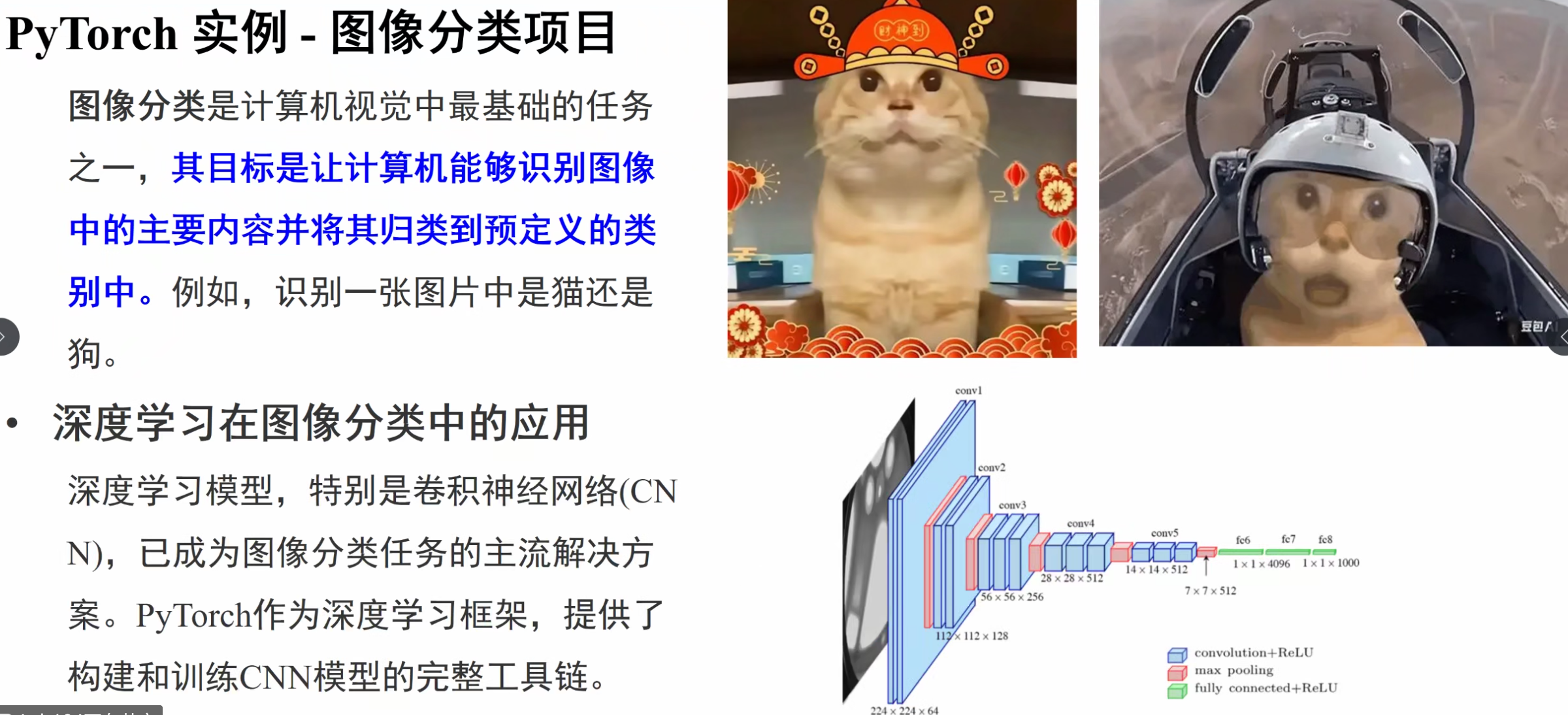
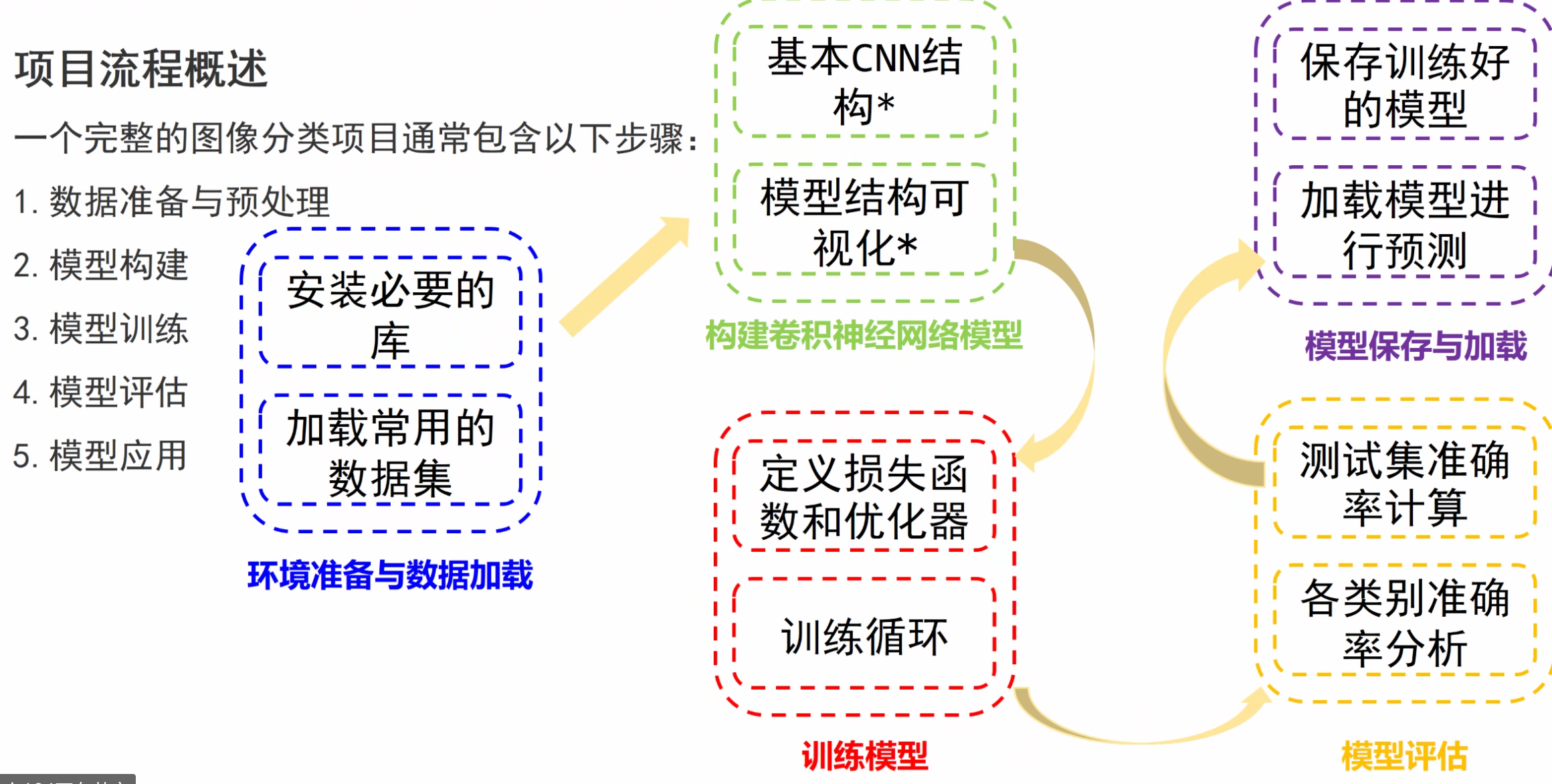
图像分类略讲